Self-test Solutions

Nestled within the chapters of Discovering Statistics Using R and RStudio (2nd edition) are questions that prompt you to think about the material. This page has the solutions to those questions.
In many cases the solutions are in the Chapter itself directly after the test. Rather than repeat these solutions, this page contains only solutions that are not already in the book
These solutions assume you have a setup code chunk at the start of your document that loads the easystats and tidyverse packages:
This document contains abridged sections from Discovering Statistics Using R and RStudio by Andy Field so there are some copyright considerations. You can use this material for teaching and non-profit activities but please do not meddle with it or claim it as your own work. See the full license terms at the bottom of the page.
Many tasks will require you to load data. You can do this in one of two ways. The easiest is to grab the data directly from the discovr package using the general code:
my_tib <- discovr::name_of_datain which you replace my_tib with the name you wish to give the data once loaded and name_of_data is the data you wish to load. In RStudio if you type discovr:: it will list the datasets available. For example, to load the data called students into a tibble called students_tib we’d execute:
students_tib <- discovr::studentsAlternatively, download the CSV file from https://www.discovr.rocks/csv/name_of_file replacing name_of_file with the name of the csv file. For example, to download students.csv use this url: https://www.discovr.rocks/csv/students.csv
Set up an RStudio project (exactly as described in Chapter 4), place the csv file in your data folder and use this general code:
in which you replace my_tib with the name you wish to give the data once loaded and name_of_file.csv is the name of the file you wish to read into here to locate the file within the project and read_csv() to read it into students.csv you would execute
Chapter 1
Self-test 1.1
Based on what you have read in this section, what qualities do you think a scientific theory should have?
A good theory should do the following:
- Explain the existing data.
- Explain a range of related observations.
- Allow statements to be made about the state of the world.
- Allow predictions about the future.
- Have implications.
Self-test 1.2
What is the difference between reliability and validity?
Validity is whether an instrument measures what it was designed to measure, whereas reliability is the ability of the instrument to produce the same results under the same conditions.
Self-test 1.3
Why is randomization important?
It is important because it rules out confounding variables (factors that could influence the outcome variable other than the factor in which you’re interested). For example, with groups of people, random allocation of people to groups should mean that factors such as intelligence, age and gender are roughly equal in each group and so will not systematically affect the results of the experiment.
Self-test 1.4
Compute the mean but excluding the score of 234.
\[ \begin{aligned} \overline{X} &= \frac{\sum_{i=1}^{n} x_i}{n} \\ \ &= \frac{22+40+53+57+93+98+103+108+116+121}{10} \\ \ &= \frac{811}{10} \\ \ &= 81.1 \end{aligned} \]
Self-test 1.5
Compute the range but excluding the score of 234.
Range = maximum score - minimum score = 121 − 22 = 99.
Self-test 1.6
Twenty-one heavy smokers were put on a treadmill at the fastest setting. The time in seconds was measured until they fell off from exhaustion: 18, 16, 18, 24, 23, 22, 22, 23, 26, 29, 32, 34, 34, 36, 36, 43, 42, 49, 46, 46, 57. Compute the mode, median, mean, upper and lower quartiles, range and interquartile range
First, let’s arrange the scores in ascending order: 16, 18, 18, 22, 22, 23, 23, 24, 26, 29, 32, 34, 34, 36, 36, 42, 43, 46, 46, 49, 57.
- The mode: The scores with frequencies in brackets are: 16 (1), 18 (2), 22 (2), 23 (2), 24 (1), 26 (1), 29 (1), 32 (1), 34 (2), 36 (2), 42 (1), 43 (1), 46 (2), 49 (1), 57 (1). Therefore, there are several modes because 18, 22, 23, 34, 36 and 46 seconds all have frequencies of 2, and 2 is the largest frequency. These data are multimodal (and the mode is, therefore, not particularly helpful to us).
- The median: The median will be the (n + 1)/2th score. There are 21 scores, so this will be the 22/2 = 11th. The 11th score in our ordered list is 32 seconds.
- The mean: The mean is 32.19 seconds:
\[ \begin{aligned} \overline{X} &= \frac{\sum_{i=1}^{n} x_i}{n} \\ \ &= \frac{16+(2\times18)+(2\times22)+(2\times23)+24+26+29+32+(2\times34)+(2\times36)+42+43+(2\times46)+49+57}{21} \\ \ &= \frac{676}{21} \\ \ &= 32.19 \end{aligned} \]
- The lower quartile: This is the median of the lower half of scores. If we split the data at 32 (not including this score), there are 10 scores below this value. The median of 10 scores is the 11/2 = 5.5th score. Therefore, we take the average of the 5th score and the 6th score. The 5th score is 22, and the 6th is 23; the lower quartile is therefore 22.5 seconds.
- The upper quartile: This is the median of the upper half of scores. If we split the data at 32 (not including this score), there are 10 scores above this value. The median of 10 scores is the 11/2 = 5.5th score above the median. Therefore, we take the average of the 5th score above the median and the 6th score above the median. The 5th score above the median is 42 and the 6th is 43; the upper quartileis therefore 42.5 seconds.
- The range: This is the highest score (57) minus the lowest (16), i.e. 41 seconds. _ The interquartile range: This is the difference between the upper and lower quartiles: 42.5 − 22.5 = 20 seconds.
Self-test 1.7
Assuming the same mean and standard deviation for the ice bucket example above, what’s the probability that someone posted a video within the first 30 days of the challenge?
As in the example, we know that the mean number of days was 39.68, with a standard deviation of 7.74. First we convert our value to a z-score: the 30 becomes (30−39.68)/7.74 = −1.25. We want the area below this value (because 30 is below the mean), but this value is not tabulated in the Appendix. However, because the distribution is symmetrical, we could instead ignore the minus sign and look up this value in the column labelled ‘Smaller Portion’ (i.e. the area above the value 1.25). You should find that the probability is 0.10565, or, put another way, a 10.57% chance that a video would be posted within the first 30 days of the challenge. By looking at the column labelled ‘Bigger Portion’ we can also see the probability that a video would be posted after the first 30 days of the challenge. This probability is 0.89435, or a 89.44% chance that a video would be posted after the first 30 days of the challenge.
Chapter 2
Self-test 2.1
In Section 1.7.3 we came across some data about the number of friends that 11 people had on Facebook. We calculated the mean for these data as 95 and standard deviation as 56.79. Calculate a 95% confidence interval for this mean. Recalculate the confidence interval assuming that the sample size was 56.
To calculate a 95% confidence interval for the mean, we begin by calculating the standard error:
\[ SE = \frac{s}{\sqrt{N}} = \frac{56.79}{\sqrt{11}}=17.12 \]
The sample is small, so to calculate the confidence interval we need to find the appropriate value of t. For this we need the degrees of freedom, N – 1. With 11 data points, the degrees of freedom are 10. For a 95% confidence interval we can look up the value in the column labelled ‘Two-Tailed Test’, ‘0.05’ in the table of critical values of the t-distribution (Appendix). The corresponding value is 2.23. The confidence interval is, therefore, given by:
\[ \begin{aligned} \text{lower boundary of confidence interval} &= \bar{X}-(2.23 \times 17.12) \\ &= 95 - (2.23 \times 17.12) \\ & = 56.82 \\ \text{upper boundary of confidence interval} &= \bar{X}+(2.23 \times 17.12) \\ &= 95 + (2.23 \times 17.12) \\ &= 133.18 \end{aligned} \]
Assuming now a sample size of 56, we need to calculate the new standard error:
\[ SE = \frac{s}{\sqrt{N}} = \frac{56.79}{\sqrt{56}}=7.59 \]
The sample is big now, so to calculate the confidence interval we can use the critical value of z for a 95% confidence interval (i.e. 1.96). The confidence interval is, therefore, given by:
\[ \begin{aligned} \text{lower boundary of confidence interval} &= \bar{X}-(1.96 \times 7.59) = 95 - (1.96 \times 7.59) = 80.1 \\ \text{upper boundary of confidence interval} &= \bar{X}+(1.96 \times 7.59) = 95 + (1.96 \times 7.59) = 109.8 \end{aligned} \]
Self-test 2.2
What are the null and alternative hypotheses for the following questions: (1) ‘Is there a relationship between the amount of gibberish that people speak and the amount of vodka jelly they’ve eaten?’ (2) ‘Does reading this chapter improve your knowledge of research methods?’
‘Is there a relationship between the amount of gibberish that people speak and the amount of vodka jelly they’ve eaten?’
- Null hypothesis: There will be no relationship between the amount of gibberish that people speak and the amount of vodka jelly they’ve eaten.
- Alternative hypothesis: There will be a relationship between the amount of gibberish that people speak and the amount of vodka jelly they’ve eaten.
‘Does reading this chapter improve your knowledge of research methods?’
- Null hypothesis: There will be no difference in the knowledge of research methods in people who have read this chapter compared to those who have not.
- Alternative hypothesis: Knowledge of research methods will be in those who have read the chapter compared to those who have not.
Self-test 2.3
Compare the plots in Figure 2.16. What effect does the difference in sample size have? Why do you think it has this effect?
The plot showing larger sample sizes has smaller confidence intervals than the plot showing smaller sample sizes. If you think back to how the confidence interval is computed, it is the mean plus or minus 1.96 times the standard error. The standard error is the standard deviation divided by the square root of the sample size (√N), therefore as the sample size gets larger, the standard error (and, therefore, confidence interval) will get smaller.
Chapter 3
Self-test 3.1
Based on what you have learnt so far, which of the following statements best reflects your view of antiSTATic? (A) The evidence is equivocal, we need more research. (B) All of the mean differences show a positive effect of antiSTATic, therefore, we have consistent evidence that antiSTATic works. (C) Four of the studies show a significant result (p < .05), but the other six do not. Therefore, the studies are inconclusive: some suggest that antiSTATic is better than placebo, but others suggest there’s no difference. The fact that more than half of the studies showed no significant effect means that antiSTATic is not (on balance) more successful in reducing anxiety than the control. (D) I want to go for C, but I have a feeling it’s a trick question.
If you follow NHST you should pick C because only four of the six studies have a ‘significant’ result, which isn’t very compelling evidence for antiSTATic.
Self-test 3.2
Now you’ve looked at the confidence intervals, which of the earlier statements best reflects your view of Dr Weeping’s potion?
I would hope that some of you have changed your mind to option B: 10 out of 10 studies show a positive effect of antiSTATic (none of the means are below zero), and even though sometimes this positive effect is not always ‘significant’, it is consistently positive. The confidence intervals overlap with each other substantially in all studies, suggesting that all studies have sampled the same population. Again, this implies great consistency in the studies: they all throw up (potential) population effects of a similar size. Look at how much of the confidence intervals are above zero across the 10 studies: even in studies for which the confidence interval includes zero (implying that the population effect might be zero) the majority of the bar is greater than zero. Again, this suggests very consistent evidence that the population value is greater than zero (i.e. antiSTATic works).
Self-test 3.3
Compute Cohen’s d for the effect of singing when a sample size of 100 was used (right-hand plot in Figure 2.21).
\[ \begin{aligned} \hat{d} &= \frac{\bar{X}_\text{singing}-\bar{X}_\text{conversation}}{\sigma} \\ &= \frac{10-12}{3} \\ &= 0.667 \end{aligned} \]
Self-test 3.4
Compute Cohen’s d for the effect in Figure 2.22. The exact mean of the singing group was 10, and for the conversation group was 10.01. In both groups the standard deviation was 3.
\[ \begin{aligned} \hat{d} &= \frac{\bar{X}_\text{singing}-\bar{X}_\text{conversation}}{\sigma} \\ &= \frac{10-10.01}{3} \\ &= -0.003 \end{aligned} \]
Self-test 3.5
Look at Figures 2.22 and Figure 2.23. Compare what we concluded about these three data sets based on p-values, with what we conclude using effect sizes.
Answer given in the text.
Self-test 3.6
Look back at Figure 3.2. Based on the effect sizes, is your view of the efficacy of the potion more in keeping with what we concluded based on p-values or based on confidence intervals?
Answer given in the text.
Self-test 3.7
Use Table 3.2 and Bayes’ theorem to calculate p(human |match).
Answer given in the text.
Self-test 3.8
What are the problems with NHST?
Answer given in the text.
Chapter 4
Self-test 4.1
Create a new project called discovr_stats in a folder of your choice on your computer. Create folders within you project directory called quarto and data.
Instructions are in the Chapter.
Self-tests 4.2-4.5, 4.7, 4.9, 4.11-4.19
ST 4.2: Create a new Quarto document and save it as metallica.qmd (for reasons that will reveal themselves).
ST 4.3: Edit the YAML of your Quarto document to contain embed-resources: true. Feel free to try applying a theme and table of contents.
ST 4.4: In the main body of your Quarto document, write a level 2 heading ‘About the band’ and then the following sentence (formatted in Normal style): This document is going to give me some practice at using Quarto via the power of Metallica.
ST 4.5: Create an object that represents your favourite band (unless it’s Metallica, in which case use your second favourite band) and that contains the names of each band member. If you don’t have a favourite band, then create an object called friends that contains the names of your five best friends. If you don’t have any friends, you have made a wise career choice in statistics.
ST 4.7: Create a code chunk in metallica.qmd directly below the YAML header (that is below the bottom —). Label it ‘setup’ and load the tidyverse package
ST 4.9: In your setup code chunk, add the code from Figure 4.30 to load the metallica data. Run the code in your setup code chunk.
ST 4.11: Insert a new code chunk (below your startup code chunk) and adapt the code above to create an object called name that contains these current and former members of Metallica: Lars Ulrich, James Hetfield, Kirk Hammett, Rob Trujillo, Jason Newsted, Cliff Burton, Dave Mustaine
ST 4.12: Add the code to create the variables from this section to your code chunk from the previous section.
ST 4.13: Add the code to create the
birth_dateanddeath_datevariables to your code chunk.
ST 4.14: Add the code to create the
current_membervariable to your code chunk
ST 4.15: Add the code to create the
instrumentvariable to your code chunk
ST 4.16: Add the code to your code chunk that collects your variables into a tibble called
metalli_tib
ST 4.17: Add a level 3 header to your Quarto document that says ‘Creating variables’. Write some notes on using
mutate()and add a code chunk that uses some of the code in this section to add and create new variables.
ST 4.18: Add a level 3 header to your Quarto document that says ‘Selecting variables’. Write some notes on using
select()and add a code chunk that uses some of the code in this section to select variables and re-order variables
ST 4.19: Add a level 3 header to your Quarto document that says ‘Filtering cases’. Write some notes on using
filter()and add a code chunk that uses some of the code in this section to filter the Metallica data
All of these tasks involve creating a .qmd file and adding things to it. You can download a complete version of this file (chapter_4_self_tests.qmd) and it’s rendered output (chapter_4_self_tests.html) from www.discovr.rocks/repository/chapter_4_self_tests.zip. Import the .qmd file into your project (and place it in the folder you’ve named quarto) and try rendering it.
Self-test 4.6
We use the tidyverse and easystats packages extensively in this book. To get these packages onto your computer, go to the R console, type
install.packages("tidyverse")then press return. You’ll see a load of red text, which is normal. When you see the prompt and a flashing cursor, typeinstall.packages("easystats")and press return. More red text will ensure. When the prompt re-appears, typeeasystats::install_suggested()and press return to install a bunch of stuff upon which easystats relies.
Instructions are in the task.
Self-test 4.8
Download the file
metallica.csvfrom www.discovr.rocks/csv/metallica.csv and save it to your data folder within your RStudio project.
Instructions are in the chapter.
Self-test 4.10
Identify the data type for each variable in Table 4.2.
-
nameis achr(character) variable -
birth_dateanddeath_datearedatevariables -
instrumentis afct(factor) variable -
current_memberis algl(logical) variable -
songs_written,net_worthandalbumsareint(integer) variables
Chapter 5
This page contains solutions that are not already in the book. If you can’t find the solution here then read the text directly following the self-test for the relevant code/answer.
Self-test 5.1
Create a tibble called
insta_tibcontaining the scores in a variable called followers
Self-test 5.2
What does a histogram show?
A histogram plots the values of observations on the horizontal x-axis, and the frequency with which each value occurs in the data set on the vertical y-axis.
Self-test 5.3
Try out some other values of binwidth and note how the plot changes.
First load the data
wish_tib <- discovr::jiminy_cricketFigure 1 shows plot using the code from the book chapter (binwidth = 5), Figure 2 uses a wider binwidth (binwidth = 15) and Figure 3 uses a narrower binwidth (binwidth = 1). Note the bars get wider as the binwidth increases, which reduces the definition. However, you don’t want the binwidth too narrow or you get gaps (as in Figure 4 which uses binwidth 0.5). You want to tweak the binwidth to a value where, to use highly technical terms, the plot is not ‘too chunky’ or ‘too gappy’ 😉.
ggplot(wish_tib, aes(x = success)) +
  geom_histogram(binwidth = 5)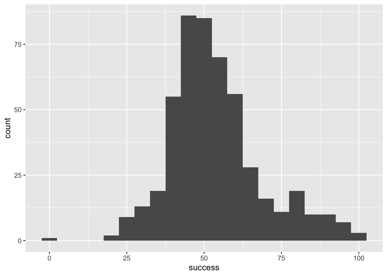
ggplot(wish_tib, aes(x = success)) +
  geom_histogram(binwidth = 15)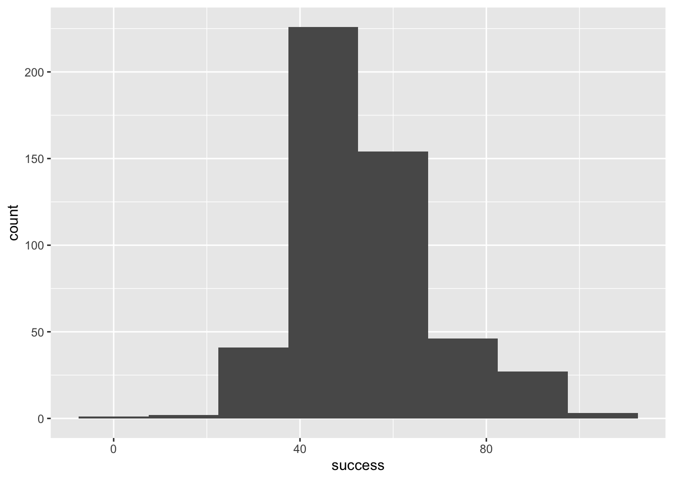
ggplot(wish_tib, aes(x = success)) +
  geom_histogram(binwidth = 1)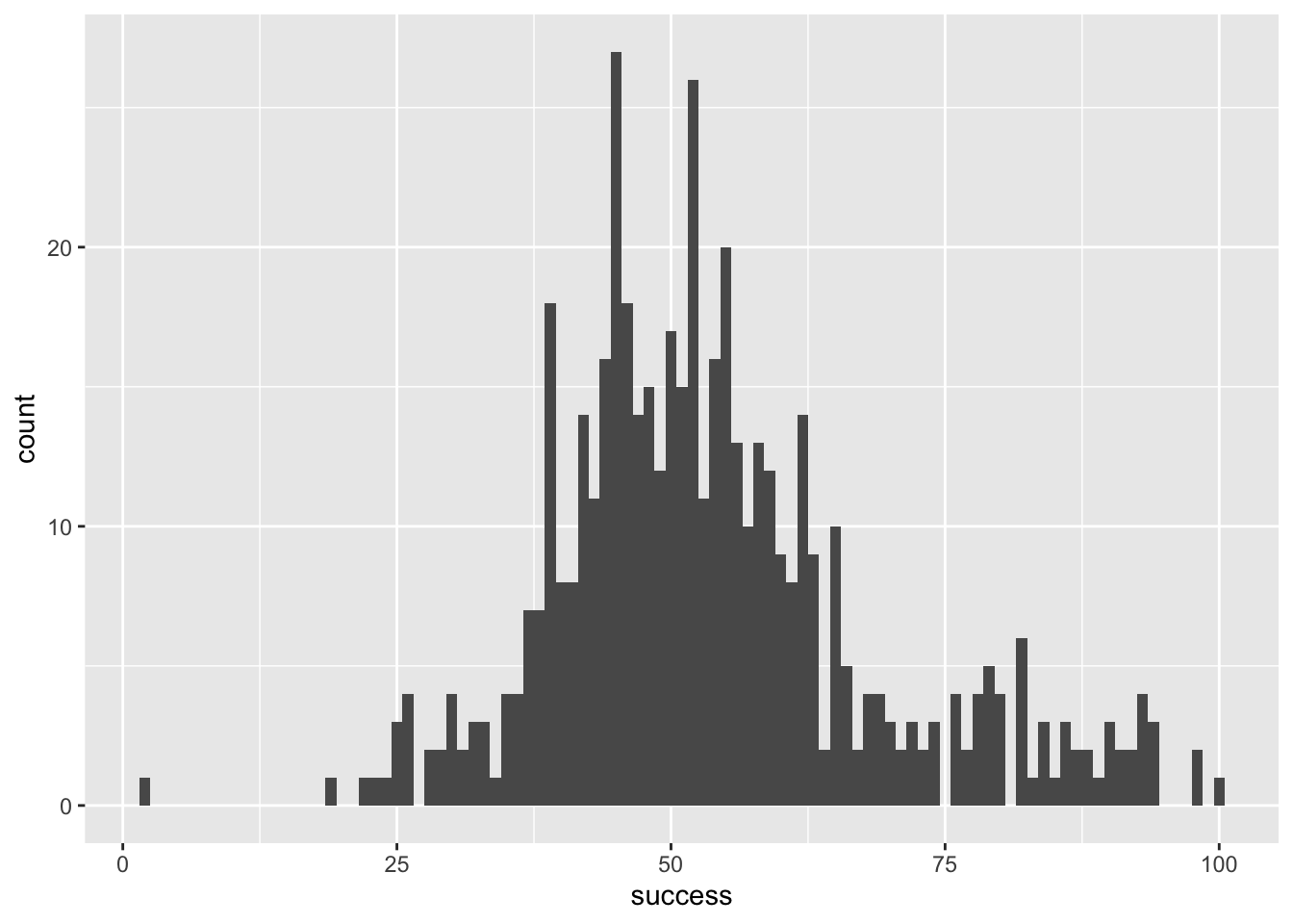
ggplot(wish_tib, aes(x = success)) +
  geom_histogram(binwidth = 0.5)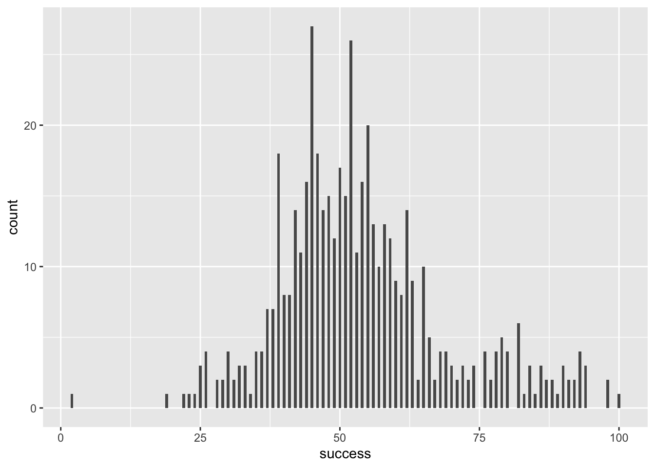
Self-test 5.4
Try out some other values of fill and colour. Take inspiration from www.color-hex.com and follow advice on accessibility
Figure 5 shows plot using the code from the book chapter (fill = "#56B4E9", colour = "#336c8b"), Figure 6 and Figure 7 use colours from the viridis pallette, which is accessible.
ggplot(wish_tib, aes(x = success)) +
  geom_histogram(binwidth = 5, fill = "#56B4E9", colour = "#336c8b")
ggplot(wish_tib, aes(x = success)) +
  geom_histogram(binwidth = 5, colour = "#7A0403FF", fill = "#C42503FF")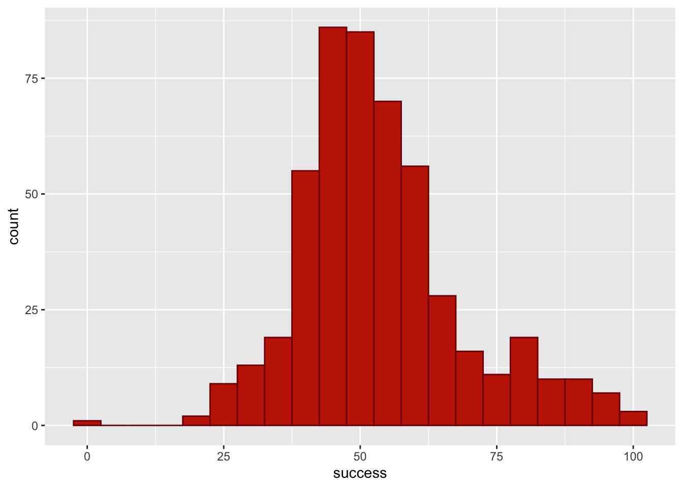
ggplot(wish_tib, aes(x = success)) +
  geom_histogram(binwidth = 5, colour = "#3E9BFEFF", fill = "#C4F134FF")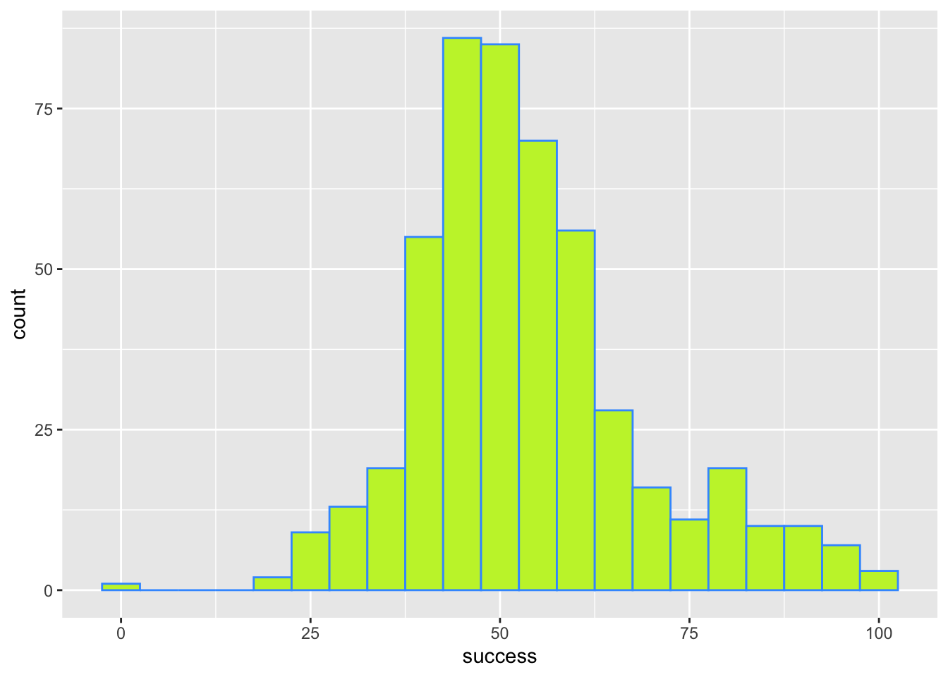
Self-test 5.5
Try out some other values of alpha
Figure 5 shows plot using the code from the book chapter (alpha = 0.2). Figure 9 uses a larger value of alpha (alpha = 0.7) to make the fill colour less transparent and Figure 10 uses a smaller value of alpha (alpha = 0.05) to make the fill colour more transparent.
ggplot(wish_tib, aes(x = success)) +
  geom_histogram(binwidth = 5, fill = "#56B4E9", colour = "#336c8b", alpha = 0.2)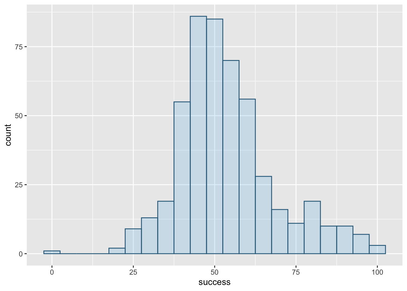
alpha = 0.2
ggplot(wish_tib, aes(x = success)) +
  geom_histogram(binwidth = 5, fill = "#56B4E9", colour = "#336c8b", alpha = 0.7)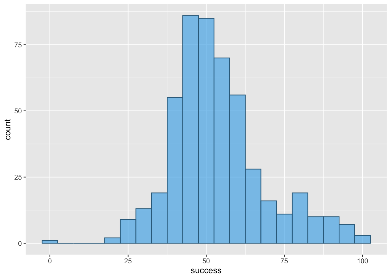
alpha = 0.7
ggplot(wish_tib, aes(x = success)) +
  geom_histogram(binwidth = 5, fill = "#56B4E9", colour = "#336c8b", alpha = 0.05)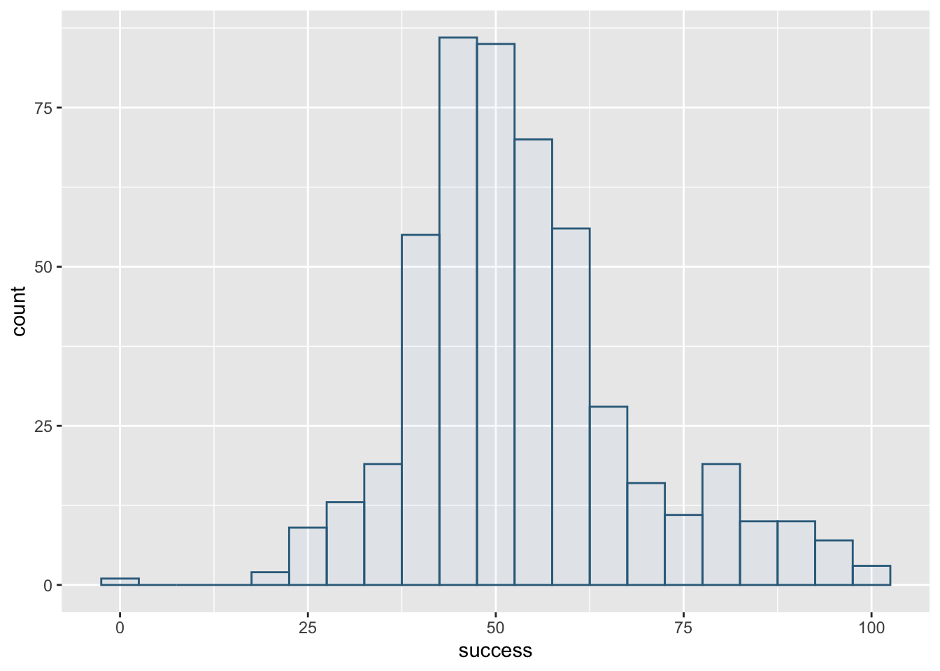
alpha = 0.05
Self-test 5.6
Change
theme_minimal()totheme_bw(),theme_classic()andtheme_dark()to see what effect these changes have on the plot
Figure 11 shows the original plot, Figure 12 applies theme_bw(), Figure 13 applies theme_classic() and Figure 14 applies theme_dark().
ggplot(wish_tib, aes(x = success)) +
  geom_histogram(binwidth = 5, fill = "#56B4E9", colour = "#336c8b", alpha = 0.2) +
  labs(y = "Frequency", x = "Success scores (0-100)") +
  theme_minimal()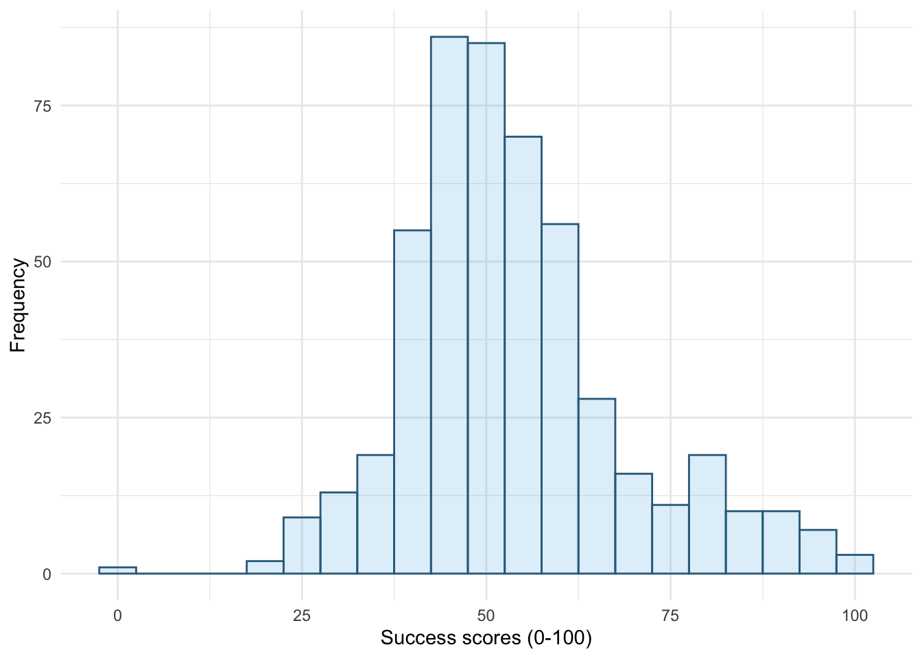
theme_minimal()
ggplot(wish_tib, aes(x = success)) +
  geom_histogram(binwidth = 5, fill = "#56B4E9", colour = "#336c8b", alpha = 0.2) +
  labs(y = "Frequency", x = "Success scores (0-100)") +
  theme_bw()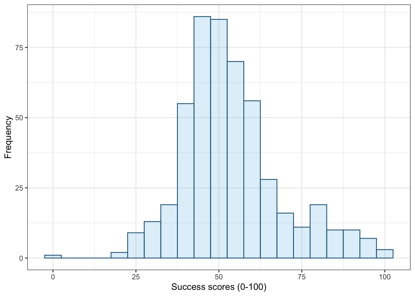
theme_bw()
ggplot(wish_tib, aes(x = success)) +
  geom_histogram(binwidth = 5, fill = "#56B4E9", colour = "#336c8b", alpha = 0.2) +
  labs(y = "Frequency", x = "Success scores (0-100)") +
  theme_classic()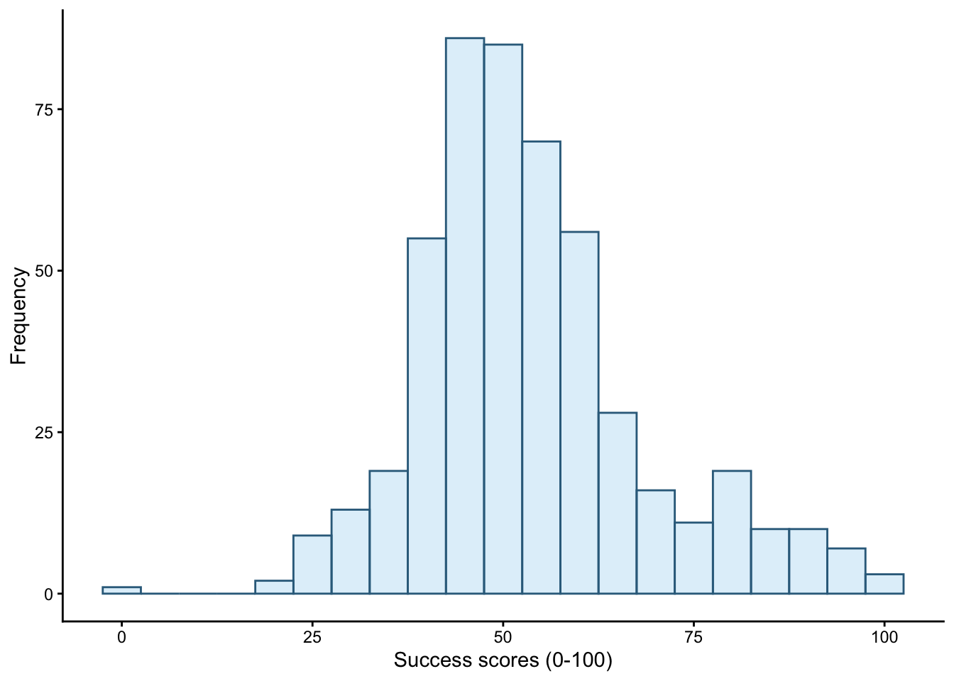
theme_classic()
ggplot(wish_tib, aes(x = success)) +
  geom_histogram(binwidth = 5, fill = "#56B4E9", colour = "#336c8b", alpha = 0.2) +
  labs(y = "Frequency", x = "Success scores (0-100)") +
  theme_dark()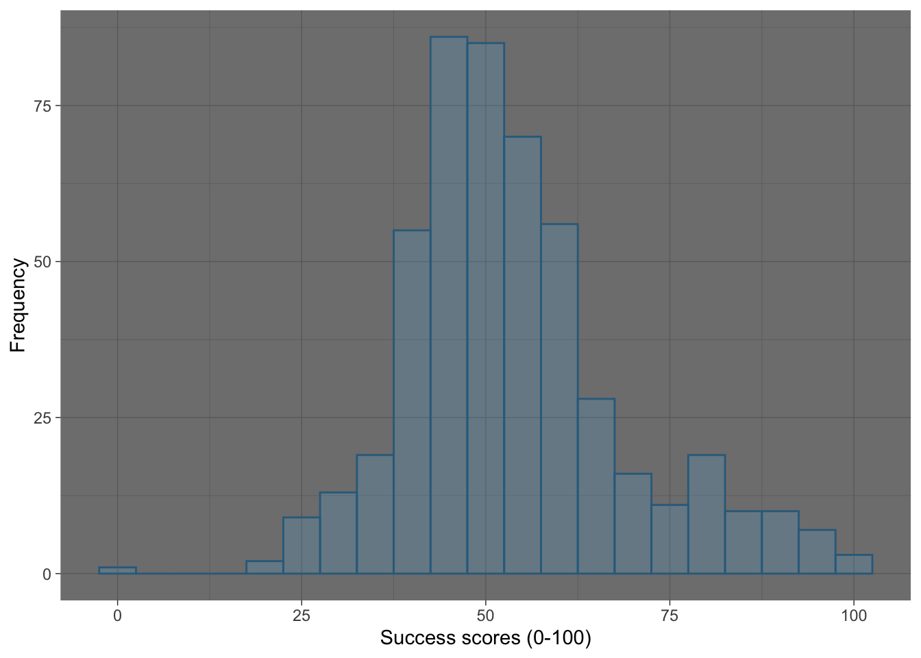
theme_dark()
Self-test 5.7
Change the order of the variables in
facet_grid()to befacet_grid(time~strategy). What effect does this have?
Figure 15 shows the original plot. Figure 16 uses facet_grid(time~strategy), notice that the plots in different columns are now in different rows and vice versa.
ggplot(wish_tib, aes(x = success)) +
  geom_histogram(binwidth = 5, fill = "#56B4E9", colour = "#336c8b", alpha =
0.2) +
  labs(y = "Frequency", x = "Success scores (0-100)") +
  facet_grid(strategy~time) +
  theme_minimal()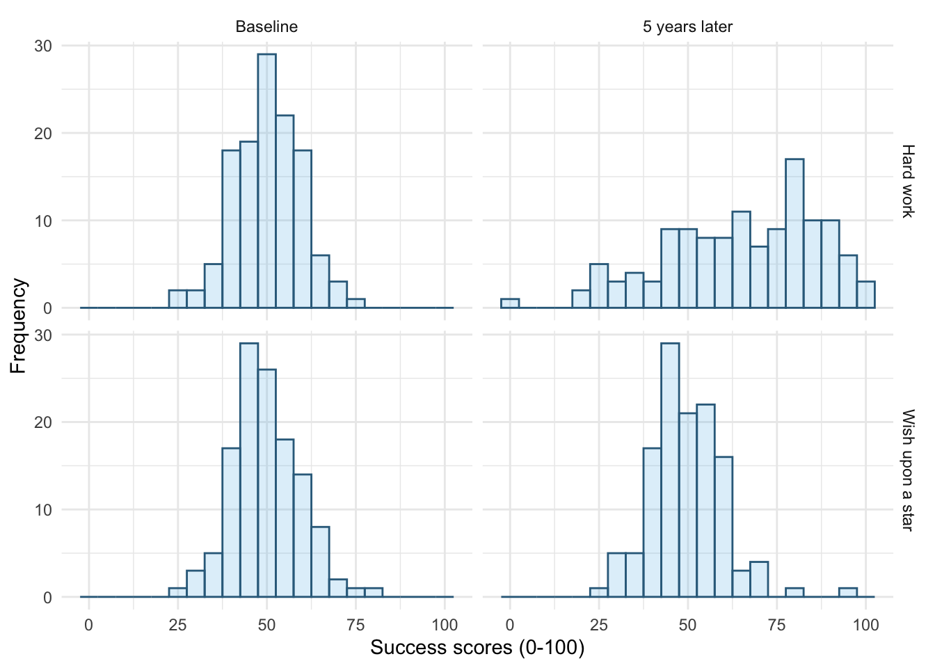
facet_grid(strategy~time)
ggplot(wish_tib, aes(x = success)) +
  geom_histogram(binwidth = 5, fill = "#56B4E9", colour = "#336c8b", alpha =
0.2) +
  labs(y = "Frequency", x = "Success scores (0-100)") +
  facet_grid(time~strategy) +
  theme_minimal()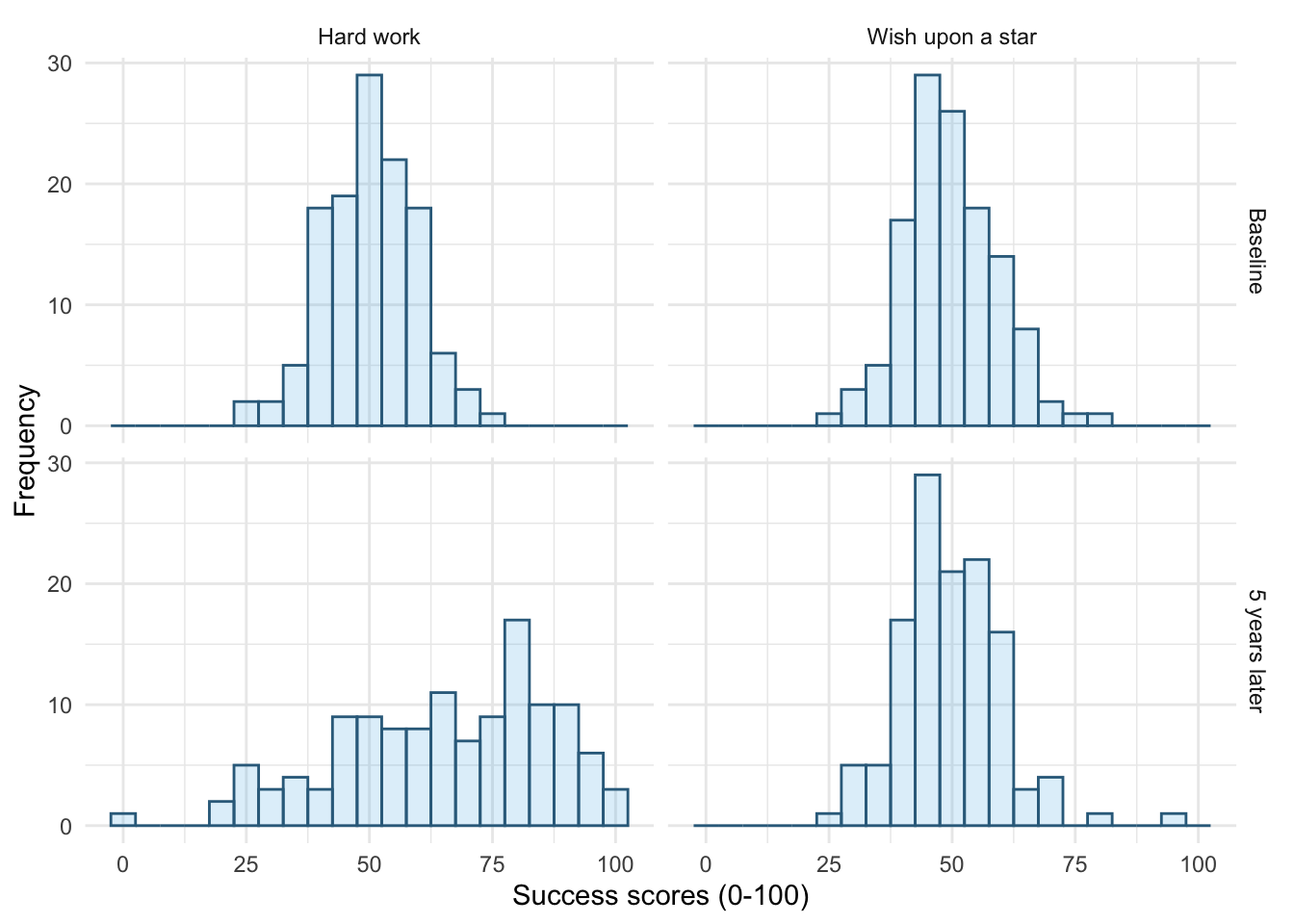
facet_grid(time~strategy)
Self-test 5.8
Try out different combinations of styles and sizes.
Figure 17 shows a plot created with the default line style (linetype = 1) and size (linewidth = 0.5).
-
Figure 18 uses
linewidth = 1, notice the line is thicker than the default. -
Figure 19 uses
linewidth = 0.25, notice the line is thinner than the default. -
Figure 20 uses
linetype = 3, notice the (default) solid line is now a dotted line. -
Figure 21 uses
linetype = 4, notice the (default) solid line is now a line made up of dot-dashes. -
Figure 22 uses
linetype = 5andlinewidth = 1. Notice the (default) solid line is now thicker, but also made up of long dashes.
ggplot(wish_tib, aes(x = success)) +
  geom_freqpoly(binwidth = 5, colour = "#336c8b") +
  labs(y = "Frequency", x = "Success scores (0-100)") +
  facet_grid(strategy~time) +
  theme_minimal()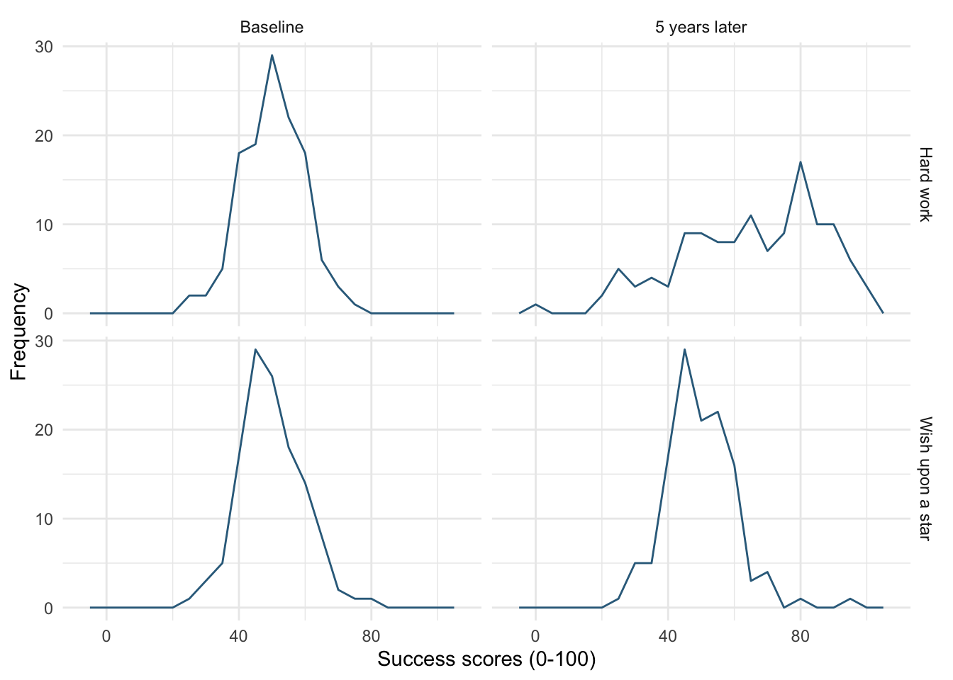
ggplot(wish_tib, aes(x = success)) +
  geom_freqpoly(binwidth = 5, colour = "#336c8b", linewidth = 1) +
  labs(y = "Frequency", x = "Success scores (0-100)") +
  facet_grid(strategy~time) +
  theme_minimal()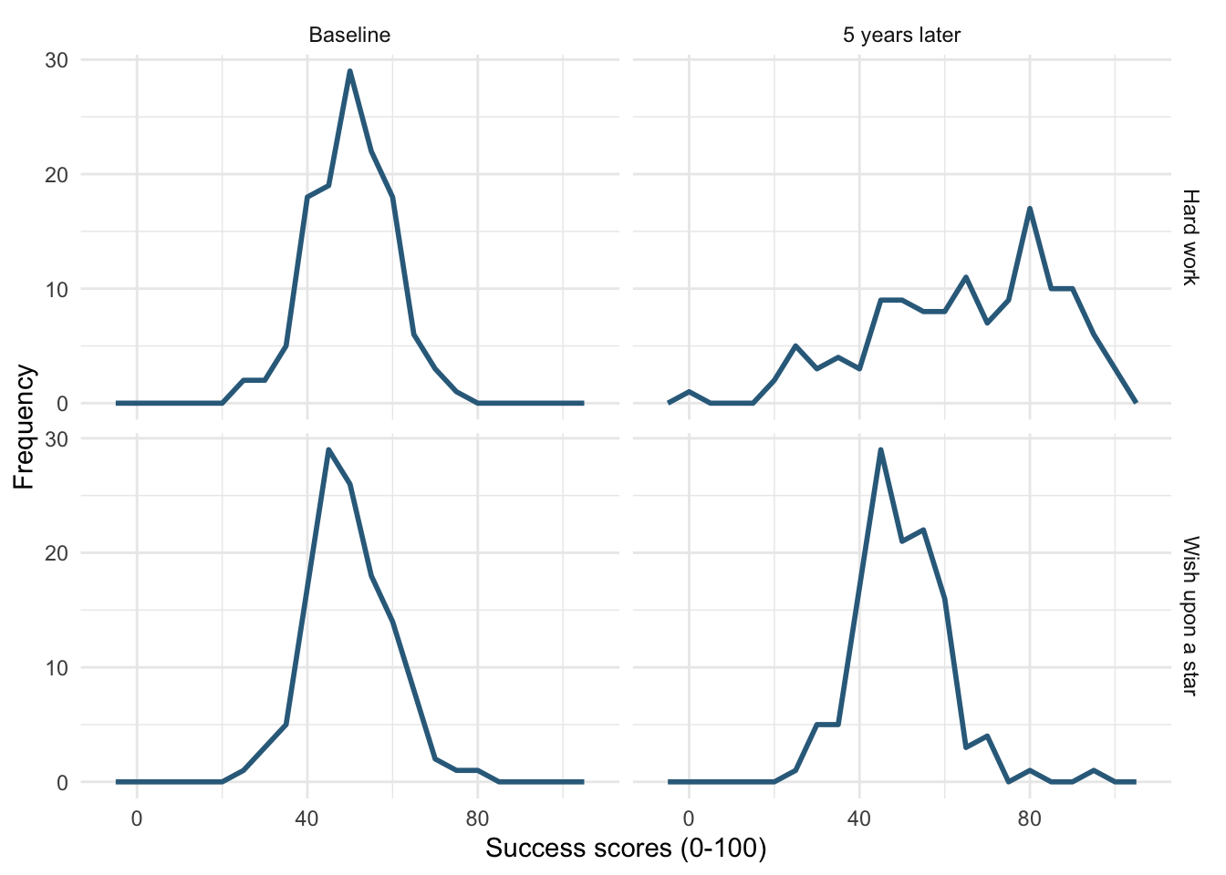
linewidth = 1
ggplot(wish_tib, aes(x = success)) +
  geom_freqpoly(binwidth = 5, colour = "#336c8b", linewidth = 0.25) +
  labs(y = "Frequency", x = "Success scores (0-100)") +
  facet_grid(strategy~time) +
  theme_minimal()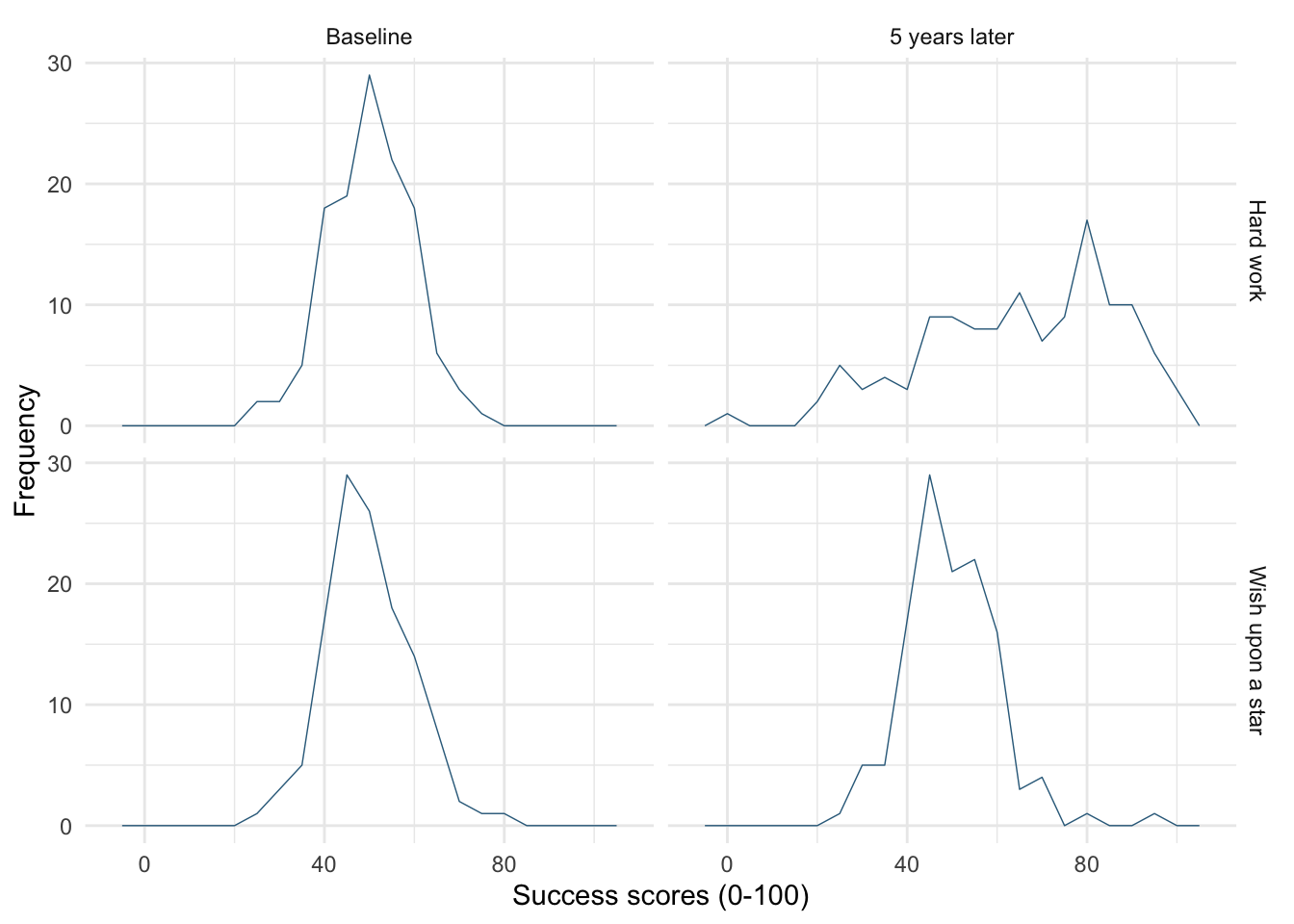
linewidth = 0.25
ggplot(wish_tib, aes(x = success)) +
  geom_freqpoly(binwidth = 5, colour = "#336c8b", linetype = 3) +
  labs(y = "Frequency", x = "Success scores (0-100)") +
  facet_grid(strategy~time) +
  theme_minimal()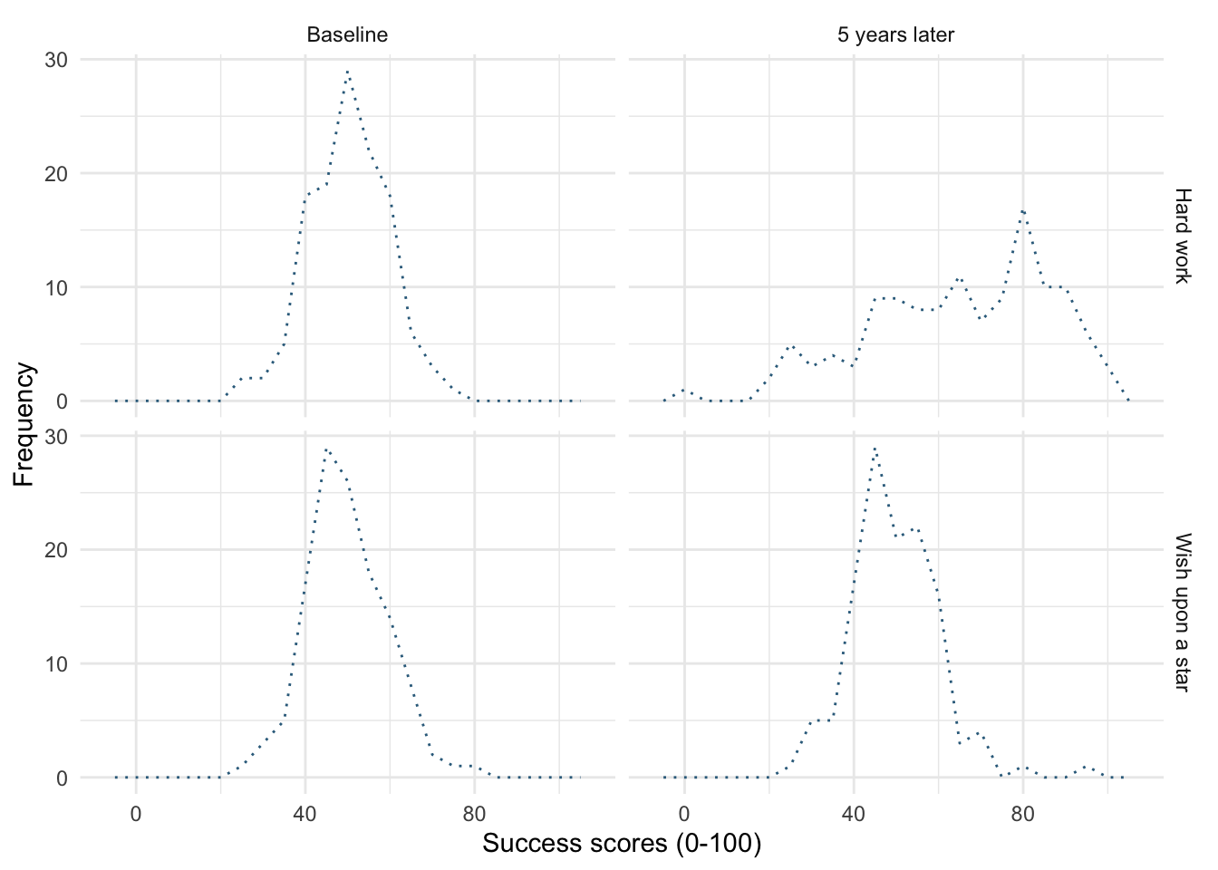
linetype = 3
ggplot(wish_tib, aes(x = success)) +
  geom_freqpoly(binwidth = 5, colour = "#336c8b", linetype = 4) +
  labs(y = "Frequency", x = "Success scores (0-100)") +
  facet_grid(strategy~time) +
  theme_minimal()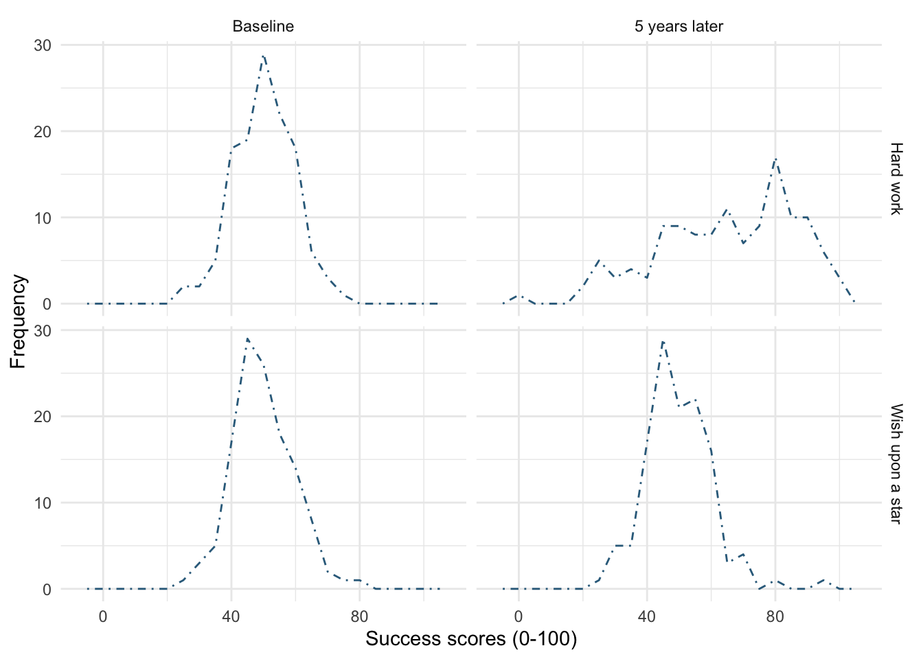
linetype = 4
ggplot(wish_tib, aes(x = success)) +
  geom_freqpoly(binwidth = 5, colour = "#336c8b", linetype = 5, linewidth = 1) +
  labs(y = "Frequency", x = "Success scores (0-100)") +
  facet_grid(strategy~time) +
  theme_minimal()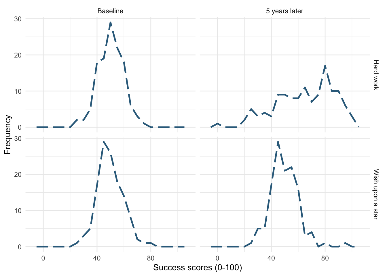
linetype = 5 and linewidth = 1
Self-test 5.11
Edit your code to replace
geom_violin() +withgeom_violin(alpha = 0.7) +Note that the violins become more transparent when you execute this updated code
Figure 23 shows the original plot. Figure 24 uses geom_violin(alpha = 0.7), note that the violins are more transparent in this plot.
ggplot(notebook_tib, aes(x = film, y = arousal, fill = gender_identity)) +
  geom_violin() +
  stat_summary(fun.data = "mean_cl_normal", geom = "pointrange", position = position_dodge(width = 0.9)) +
  coord_cartesian(ylim = c(0, 50)) +
  scale_y_continuous(breaks = seq(0, 50, 5)) +
  labs(x = "Type of film", y = "Arousal (out of 100)", fill = "Gender identity") +
  theme_minimal()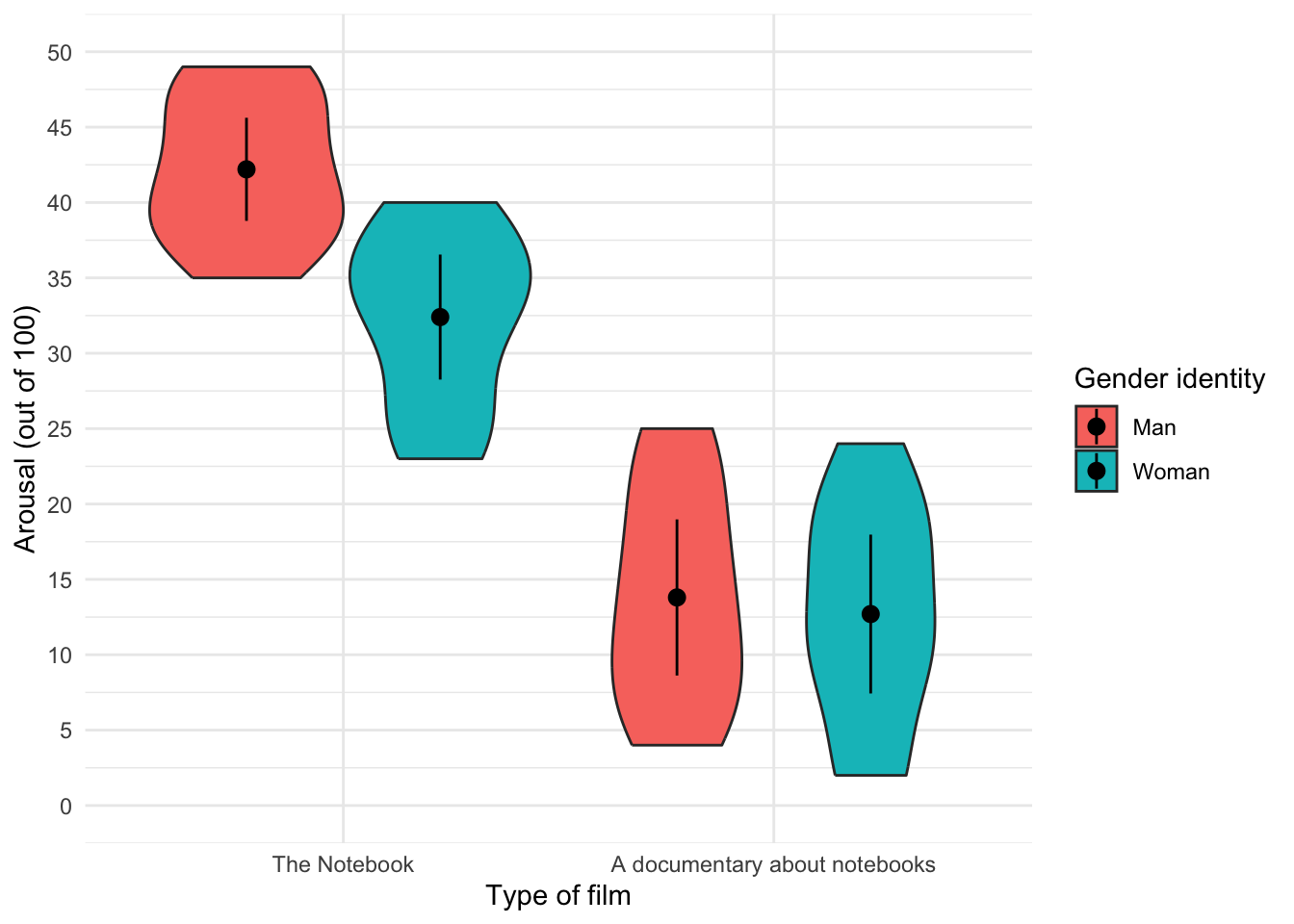
ggplot(notebook_tib, aes(x = film, y = arousal, fill = gender_identity)) +
  geom_violin(alpha = 0.7) +
  stat_summary(fun.data = "mean_cl_normal", geom = "pointrange", position = position_dodge(width = 0.9)) +
  coord_cartesian(ylim = c(0, 50)) +
  scale_y_continuous(breaks = seq(0, 50, 5)) +
  labs(x = "Type of film", y = "Arousal (out of 100)", fill = "Gender identity") +
  theme_minimal()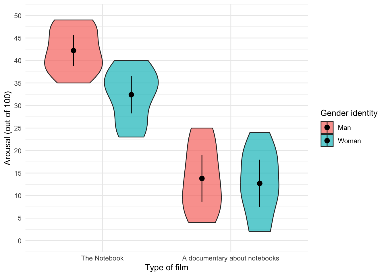
geom_violin(alpha = 0.7)
Chapter 6
This page contains solutions that are not already in the book. If you can’t find the solution here then read the text directly following the self-test for the relevant code/answer.
Self-test 6.1
Compute the mean and sum of squared error for the new data set.
First we need to compute the mean:
\[ \begin{aligned} \overline{X} &= \frac{\sum_{i=1}^{n} x_i}{n} \\ \ &= \frac{1+3+10+3+2}{5} \\ \ &= \frac{19}{5} \\ \ &= 3.8 \end{aligned} \]
Compute the squared errors as in Table 1.
| Score | Error (score - mean) | Error squared |
|---|---|---|
| 1 | -2.8 | 7.84 |
| 3 | -0.8 | 0.64 |
| 10 | 6.2 | 38.44 |
| 3 | -0.8 | 0.64 |
| 2 | -1.8 | 3.24 |
The sum of squared errors is:
\[ \begin{aligned} \ SS &= 7.84 + 0.64 + 38.44 + 0.64 + 3.24 \\ \ &= 50.8 \\ \end{aligned} \]
Self-test 6.5
Compute the mean and variance of the attractiveness ratings. Now compute them for the 5%, 10% and 20% trimmed data
Mean and variance
Compute the squared errors as follows. First let’s get a table of squared errors for each case (Table 2).
| Score | Error (score - mean) | Error squared |
|---|---|---|
| 0 | -6 | 36 |
| 0 | -6 | 36 |
| 3 | -3 | 9 |
| 4 | -2 | 4 |
| 4 | -2 | 4 |
| 5 | -1 | 1 |
| 5 | -1 | 1 |
| 6 | 0 | 0 |
| 6 | 0 | 0 |
| 6 | 0 | 0 |
| 6 | 0 | 0 |
| 7 | 1 | 1 |
| 7 | 1 | 1 |
| 7 | 1 | 1 |
| 8 | 2 | 4 |
| 8 | 2 | 4 |
| 9 | 3 | 9 |
| 9 | 3 | 9 |
| 10 | 4 | 16 |
| 10 | 4 | 16 |
| 120 | 152 |
To calculate the mean of the attractiveness ratings we use the equation (and the sum of the first column in Table 2):
\[ \begin{aligned} \overline{X} &= \frac{\sum_{i=1}^{n} x_i}{n} \\ \ &= \frac{120}{20} \\ \ &= 6 \end{aligned} \]
To calculate the variance we use the sum of squares (the sum of the values in the final column of the Table 2) and this equation:
\[ \begin{aligned} \ s^2 &= \frac{\text{sum of squares}}{n-1} \\ \ &= \frac{152}{19} \\ \ &= 8 \end{aligned} \]
5% trimmed mean and variance
Next, let’s calculate the mean and variance for the 5% trimmed data. We basically do the same thing as before but delete 1 score at each extreme (there are 20 scores and 5% of 20 is 1). Compute the squared errors as in Table 3.
| Score | Error (score - mean) | Error squared |
|---|---|---|
| 0 | -6.11 | 37.33 |
| 3 | -3.11 | 9.67 |
| 4 | -2.11 | 4.45 |
| 4 | -2.11 | 4.45 |
| 5 | -1.11 | 1.23 |
| 5 | -1.11 | 1.23 |
| 6 | -0.11 | 0.01 |
| 6 | -0.11 | 0.01 |
| 6 | -0.11 | 0.01 |
| 6 | -0.11 | 0.01 |
| 7 | 0.89 | 0.79 |
| 7 | 0.89 | 0.79 |
| 7 | 0.89 | 0.79 |
| 8 | 1.89 | 3.57 |
| 8 | 1.89 | 3.57 |
| 9 | 2.89 | 8.35 |
| 9 | 2.89 | 8.35 |
| 10 | 3.89 | 15.13 |
| 110 | 99.74 |
To calculate the mean of the attractiveness ratings we use the equation (and the sum of the first column in Table 3):
\[ \begin{aligned} \overline{X} &= \frac{\sum_{i=1}^{n} x_i}{n} \\ \ &= \frac{110}{18} \\ \ &= 6.11 \end{aligned} \]
To calculate the variance we use the sum of squares (the sum of the values in the final column of Table 3) and this equation:
\[ \begin{aligned} \ s^2 &= \frac{\text{sum of squares}}{n-1} \\ \ &= \frac{99.74}{17} \\ \ &= 5.87 \\ \end{aligned} \]
10% trimmed mean and variance
Next, let’s calculate the mean and variance for the 10% trimmed data. To do this we need to delete 2 scores from each extreme of the original data set (there are 20 scores and 10% of 20 is 2). Compute the squared errors as in Table 4.
| Score | Error (score - mean) | Error squared |
|---|---|---|
| 3 | -3.25 | 10.56 |
| 4 | -2.25 | 5.06 |
| 4 | -2.25 | 5.06 |
| 5 | -1.25 | 1.56 |
| 5 | -1.25 | 1.56 |
| 6 | -0.25 | 0.06 |
| 6 | -0.25 | 0.06 |
| 6 | -0.25 | 0.06 |
| 6 | -0.25 | 0.06 |
| 7 | 0.75 | 0.56 |
| 7 | 0.75 | 0.56 |
| 7 | 0.75 | 0.56 |
| 8 | 1.75 | 3.06 |
| 8 | 1.75 | 3.06 |
| 9 | 2.75 | 7.56 |
| 9 | 2.75 | 7.56 |
| 100 | 46.96 |
To calculate the mean of the attractiveness ratings we use the equation (and the sum of the first column in Table 4):
\[ \begin{aligned} \overline{X} &= \frac{\sum_{i=1}^{n} x_i}{n} \\ \ &= \frac{100}{16} \\ \ &= 6.25 \end{aligned} \]
To calculate the variance we use the sum of squares (the sum of the values in the final column of Table 4) and this equation:
\[ \begin{aligned} \ s^2 &= \frac{\text{sum of squares}}{n-1} \\ \ &= \frac{46.96}{15} \\ \ &= 3.13 \\ \end{aligned} \]
20% trimmed mean and variance
Finally, let’s calculate the mean and variance for the 20% trimmed data. To do this we need to delete 4 scores from each extreme of the original data set (there are 20 scores and 20% of 20 is 4). Compute the squared errors as in Table 5.
| Score | Error (score - mean) | Error squared |
|---|---|---|
| 4 | -2.25 | 5.06 |
| 5 | -1.25 | 1.56 |
| 5 | -1.25 | 1.56 |
| 6 | -0.25 | 0.06 |
| 6 | -0.25 | 0.06 |
| 6 | -0.25 | 0.06 |
| 6 | -0.25 | 0.06 |
| 7 | 0.75 | 0.56 |
| 7 | 0.75 | 0.56 |
| 7 | 0.75 | 0.56 |
| 8 | 1.75 | 3.06 |
| 8 | 1.75 | 3.06 |
| 75 | 16.22 |
To calculate the mean of the attractiveness ratings we use the equation (and the sum of the first column in Table 5):
\[ \begin{aligned} \overline{X} &= \frac{\sum_{i=1}^{n} x_i}{n} \\ \ &= \frac{75}{12} \\ \ &= 6.25 \end{aligned} \]
To calculate the variance we use the sum of squares (the sum of the values in the final column of Table 5) and this equation:
\[ \begin{aligned} \ s^2 &= \frac{\text{sum of squares}}{n-1} \\ \ &= \frac{16.22}{11} \\ \ &= 1.47 \\ \end{aligned} \]
Chapter 7
This page contains solutions that are not already in the book. If you can’t find the solution here then read the text directly following the self-test for the relevant code/answer.
Self-test 7.1
Did creativity cause success in the World’s Biggest Liar competition?
No, correlation never implies causality! Statistically speaking there is an association between creativity and competition success but we can no more conclude that creativity caused success than we can that success in the competition caused creativity.
Self-test 7.2
Conduct a Pearson correlation analysis of the advert data from the beginning of the chapter
Input the data using the code below (the data are shown in Table 6).
| adverts | packets |
|---|---|
| 5 | 8 |
| 4 | 9 |
| 4 | 10 |
| 6 | 13 |
| 8 | 15 |
Now we’ll fit the model. Table 7 shows the output, which matches the calculations in the book. There was a non-significant (because of the tiny sample size) but massive positive association between the number of adverts watched and the number of packets of crisps eaten, \(r\) = 0.87 (-0.05, 0.99), t(3) = 3.07, p = 0.054
Chapter 8
This page contains solutions that are not already in the book. If you can’t find the solution here then read the text directly following the self-test for the relevant code/answer.
Self-test 8.2
Once you have read Section 8.8, fit a linear model first with all the cases included and then with case 30 filtered out
Load the data using (see Tip 1):
dfbeta_tib <- discovr::df_betaThe data contain a variable that identifies the case, the a predictor(imaginatively labelled x) and an outcome (labelled y). The parameter estimates for the model with all cases is shown in Table 8, whereas the model with case 30 excluded is in Table 9.
| Parameter | Coefficient | SE | 95% CI | t(28) | p |
|---|---|---|---|---|---|
| (Intercept) | 29.00 | 0.99 | (26.97, 31.03) | 29.24 | < .001 |
| x | -0.90 | 0.06 | (-1.02, -0.79) | -16.17 | < .001 |
| Parameter | Coefficient | SE | 95% CI | t(27) | p |
|---|---|---|---|---|---|
| (Intercept) | 31.00 | 7.78e-16 | (31.00, 31.00) | 39836625360849056 | < .001 |
| x | -1.00 | 4.31e-17 | (-1.00, -1.00) | -23202225725833228 | < .001 |
Self-test 8.6
How many albums would be sold if we spent £666,000 on advertising the latest album by Deafheaven?
Remember that advertising budget is in thousands, so we need to put £666 into the model (not £666,000). The b-values come from the output in the chapter:
\[ \begin{aligned} \widehat{\text{sales}}_i &= \hat{b}_0 + \hat{b}_1\text{advertising}_i \\ \widehat{\text{sales}}_i &= 134.14 + (0.096 \times \text{advertising}_i) \\ \widehat{\text{sales}}_i &= 134.14 + (0.096 \times 666) \\ \widehat{\text{sales}}_i &= 198.08 \end{aligned} \]
Chapter 9
All of the self tests for this chapter are answered within the book - please read the text directly following the self-test.
Chapter 10
This page contains solutions that are not already in the book. If you can’t find the solution here then read the text directly following the self-test for the relevant code/answer.
Self-test 10.2
Assuming you did the previous self-test, compare the table of coefficients that you got with those in Output 10.3
This self-test is so you can check that your output matches Output 10.3
Self-test 10.2
Refit the model using a non-robust estimator:
lavaan::sem(infidelity_mod, data = infidelity_tib, missing = "FIML")
# load the data

infidelity_tib <- discovr::lambert_2012

infidelity_mod <- 'phys_inf ~ c*ln_porn + b*commit
commit ~ a*ln_porn
indirect_effect := a*b
total_effect := c + (a*b)
'

infidelity_fit <- lavaan::sem(infidelity_mod, data = infidelity_tib, missing = "FIML")

model_parameters(infidelity_fit) |>
display()| Link | Coefficient | SE | 95% CI | z | p |
|---|---|---|---|---|---|
| phys_inf ~ ln_porn (c) | 0.46 | 0.19 | (0.08, 0.84) | 2.38 | 0.017 |
| phys_inf ~ commit (b) | -0.27 | 0.06 | (-0.38, -0.16) | -4.64 | < .001 |
| commit ~ ln_porn (a) | -0.47 | 0.21 | (-0.89, -0.05) | -2.22 | 0.027 |
| To | Coefficient | SE | 95% CI | z | p |
|---|---|---|---|---|---|
| (indirect_effect) | 0.13 | 0.06 | (2.61e-03, 0.25) | 2.00 | 0.045 |
| (total_effect) | 0.59 | 0.20 | (0.20, 0.98) | 2.95 | 0.003 |
Chapter 11
All of the self tests for this chapter are answered within the book - please read the text directly following the self-test.
Chapter 12
All of the self tests for this chapter are answered within the book - please read the text directly following the self-test.
Chapter 13
All of the self tests for this chapter are answered within the book - please read the text directly following the self-test.
Chapter 14
All of the self tests for this chapter are answered within the book - please read the text directly following the self-test.
Chapter 15
All of the self tests for this chapter are answered within the book - please read the text directly following the self-test.
Chapter 16
This page contains solutions that are not already in the book. If you can’t find the solution here then read the text directly following the self-test for the relevant code/answer.
Self-test 16.4
What is the difference between a main effect and an interaction?
A main effect is the unique effect of a predictor variable (orindependent variable) on an outcome variable. In this context it can be the effect of strategy, charisma or looks on their own. So, in the case of strategy, the main effect is the difference between the average ratings of all dates that played hard to get (irrespective of their attractiveness or charisma) and all dates that acted typically (irrespective of their attractiveness or charisma).
The main effect of looks would be the mean rating given to all attractive dates (irrespective of their charisma, or whether they played hard to get or not), compared to the average rating given to all average-looking dates (irrespective of their charisma, or whether they played hard to get or not) and the average rating of all ugly dates (irrespective of their charisma, or whether they played hard to get or acted normally).
An interaction, on the other hand, looks at the combined effect of two or more variables: for example, were the average ratings of attractive, ugly and average-looking dates different when those dates played hard to get compared to when they did not?
Chapter 17
All of the self tests for this chapter are answered within the book - please read the text directly following the self-test.
Chapter 18
All of the self tests for this chapter are answered within the book - please read the text directly following the self-test.
Chapter 19
All of the self tests for this chapter are answered within the book - please read the text directly following the self-test.