install.packages("discovr")discovr
What is discovr?
The discovr package contains resources for my 2026 textbook Discovering Statistics using R and RStudio, which can be ordered from SAGE publications. The discovr package includes all datasets as well as interactive coding tutorials written using learnr that teach discovr package is free and offered to support tutors and students using my textbook.
To use discovr you first need to install ![]() and familiarise yourself with
and familiarise yourself with ![]() and good workflow practice. I recommend working through this playlist of tutorials on how to install, set up and work within
and good workflow practice. I recommend working through this playlist of tutorials on how to install, set up and work within ![]() before starting the interactive tutorials.
before starting the interactive tutorials.
NoteWhat are
If you’re using a textbook about
Contents of discovr
The tutorials are named to correspond (roughly) to the relevant chapter of the book. For example, discovr_04 would be a good tutorial to run alongside teaching related to chapter 4, and so on. Some longer chapters have several tutorials that break the content into more manageable chunks.
-
discovr_01: Introducing,  and Quarto: What is R, tour of RStudio and Quarto, getting help, installing packages, coding style and loading packages.
 -
discovr_02: Code fundamentals: Functions and objects, packages and functions, style, data types. -
discovr_03: The tidyverse: tidy and messy data, tibbles, adding and selecting variables, filtering cases. -
discovr_04: Summarizing data: mean, median, variance, standard deviation, interquartile range, normal and bootstrap confidence intervals, tables of summary statistics. Includes an interactive app demonstrating what a confidence interval is. -
discovr_05: Visualizing data. The ggplot2 package, boxplots, plotting means, violin plots, scatterplots, grouping by colour, grouping using facets, adjusting scales, adjusting positions.” -
discovr_06: The beast of bias. Restructuring data from messy to tidy format (and back). Spotting outliers using histograms and boxplots. Calculating z-scores (standardizing scores). Writing your own function. Using z-scores to detect outliers. Q-Q plots. Calculating skewness, kurtosis and the number of valid cases. Grouping summary statistics by multiple categorical/grouping variables. -
discovr_07: Associations. Plotting data with GGally. Pearson’s r, Spearman’s Rho, Kendall’s tau, robust correlations. Usingdisplay()to round output more flexibly. -
discovr_08: The general linear model (GLM). Visualizing the data, fitting GLMs with one and two predictors. Viewing model parameters with broom, model parameters, standard errors, confidence intervals, fit statistics, significance. -
discovr_09: Categorical predictors with two categories (comparing two means). Comparing two independent means, comparing two related means, effect sizes, robust comparisons of means (independent and related), Bayes factors and estimation (independent and related means). -
discovr_10: Moderation and mediation. Centring variables (grand mean centring), specifying interaction terms, moderation analysis, simple slopes analysis, Johnson-Neyman intervals, mediation with one predictor, direct and indirect effects, mediation usinglavaan. -
discovr_11: Comparing several means. Essentially ‘One-way independent ANOVA’ but taught using a general linear model framework. Covers setting contrasts (dummy coding, contrast coding, and linear and quadratic trends), the F-statistic and Welch’s robust F, robust parameter estimation, heteroscedasticity-consistent tests of parameters, robust tests of means based on trimmed data, post hoc tests. -
discovr_12: Linear models involving continuous and categorical predictors. The first example looks at the case o moderation (non-paralell slopes models), whereas the second explores comparing means adjusted for other variables (a parallel slopes model or ‘Analysis of Covariance (ANCOVA)’). The tutorial covers setting contrasts, fitting the models, evaluating effects using F-statistics based on Type III sums of squares and diagnostic plots, and interpretting the model using heteroscedasticity-consistent tests of parameters and post hoc tests. -
discovr_13: Factorial designs. Fitting models for two-way factorial designs (independent measures) usinglm(). This tutorial builds on previous ones to show how models can be fit with two categorical predictors to look at the interaction between them. We look at fitting the models, setting contrasts for the two categorical predictors, interaction plots, simple effects analysis, diagnostic plots and robust models. -
discovr_13_afex: Factorial designs. Fitting models for two-way factorial designs (independent measures) using theafexpackage. This tutorial takes an ANOVA approach to factorical designs. We look at fitting the models, interaction plots, simple effects analysis, diagnostic plots, partial omega-squared and robust models. -
discovr_14: Multilevel models. This tutorial looks at fitting multilevel models using theglmmTMBpackage (all code will also work withlme4). It begins with an optional section on checking and coding categorical variables before moving on to show you how to fit and interpret a multilevel model. We also look briefly at thepurrrpackage. -
discovr_15: Repeated measures designs. Fitting models for one- and two-way repeated measures designs using theafexpackage. This tutorial builds on previous ones to show how models can be fit with one or two categorical predictors when these variables have been manipulated within the same entities. We look at fitting the models, setting contrasts for the categorical predictors, obtaining estimated marginal means, interaction plots, simple effects analysis, diagnostic plots and robust models. -
discovr_15_growth: Modelling change over time. Growth models using multilevel modelling and theglmmTMBpackage. (All code will also work withlme4.) First we explore growth over time by building up a model to include a random intercept and slope for time. We then model non-linear change using both an exponential effect of time and a polynomials. We then extend the model to an example based on a clinical trial in which a fixed effect of an intervention moderates change over time. -
discovr_15_mlm: Repeated measures designs. Fitting models for one- and two-way repeated measures designs using a multilevel model framework usingglmmTMB. (All code will also work withlme4.) The examples matchdiscovr_15but the modelling approach differs. This tutorial builds on previous ones to show how models can be fit with one or two categorical predictors when these variables have been manipulated within the same entities. We look at fitting the models, setting contrasts for the categorical predictors and diagnostic plots. -
discovr_16: Mixed designs. Fitting models for mixed designs using theafexpackage. This tutorial builds on previous ones to show how models can be fit with one or two categorical predictors when at least one of these variables has been manipulated within the same entities and at least one other has been manipulated using different entities. We look at fitting the models, setting contrasts for the categorical predictors, obtaining estimated marginal means, and interaction plots. -
discovr_17: Exploratory factor analysis (EFA). This tutorial looks at using exploratory factor analysis in the context of questionnaire design. It covers factor analysis, parallel analysis and reliability analysis using MacDonald’s Omega.”. -
discovr_18: Categorical variables. Entering categorical data, contingency tables, associations between categorical variables, the chi-square test, standardized residuals, Fisher’s exact test. -
discovr_19: Categorical outcomes (logistic regression). This tutorial builds on previous ones to show how the general linear model model extends to situations where you want to predict a binary outcome (logistic regression). We look at fitting the models and interpreting the odds ratio. -
discovr_19_xmas: Christmas edition ofdiscovr_19to match the lecture I give https://youtu.be/yniFrp8vQLQ?si=DaUVAmAL6sZQ2tkT. -
discovr_bayes: Bayesian taster tutorial. This tutorial offers a taster of Bayesian statistics by showing how to estimate models from other tutorials within a Bayesian framework usingrstanarm. We also look at Bayes factors. The tutorial includes five examples of linear models: (1) predicting a continuous outcome from several continuous predictors; (2) comparing two means; (3) comparing multiple means; (4) comparing means adjusted for a covariate (ANCOVA); and (5) predicting a continuous outcome from two continuous predictors (a factorial design).
Installing discovr
The current released version is available from CRAN:
All tutorials were updated over summer 2025 but the package is in constant (minor) development. To get the most recent version install it from github.
if(!require(remotes)){
  install.packages('remotes')
}

remotes::install_github("profandyfield/discovr")
Running a tutorial
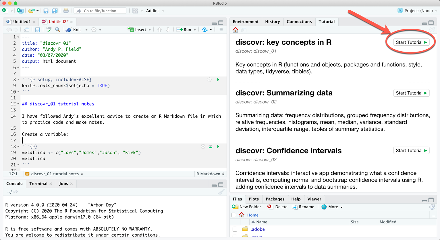
In RStudio Version 1.3 onwards there is a tutorial pane. Having executed
A list of tutorials appears in this pane. Scroll through them and click on the  button to run the tutorial:
Alternatively, to run a particular tutorial from the console execute:
library(discovr)
learnr::run_tutorial("name_of_tutorial", package = "discovr")
and replace “name of tutorial” with the name of the tutorial you want to run. For example, to run tutorial 2 execute:
learnr::run_tutorial("discovr_02", package = "discovr")The name of each tutorial is in bold in the list above. Once the command to run the tutorial is executed it will spring to life in a web browser.
Suggested workflow
The tutorials are self-contained (you practice code in code boxes) so you don’t need to use RStudio at the same time. However, to get the most from them I would recommend that you create an RStudio project and within that open (and save) a new Quarto file each time to work through a tutorial. Within that Quarto file, replicate parts of the code from the tutorial (in code chunks) and write notes about what you have done, and to reflect on things that you have struggled with, or note useful tips to help you remember things. Basically, write a learning journal. This workflow has the advantage of not just teaching you the code that you need to do certain things, but also provides practice in using RStudio itself.
Here’s a video explaining how I suggest using the tutorials.
Other resources
- The tutorials typically follow examples described in detail in Discovering Statistics using R and RStudio. That book covers the theoretical side of the statistical models, and has more depth on conducting and interpreting the models in these tutorials.
- If any of the statistical content doesn’t make sense, you could try my more introductory book An adventure in statistics.
- There are free lectures and screencasts on my YouTube channel.
- There are free statistical resources on my websites www.discoveringstatistics.com.