Oliver Twisted

Oliver, like the more famous fictional London urchin, asks ‘Please, Sir, can I have some more?’ Unlike Master Twist though, Master Twisted always wants more statistics information. Who wouldn’t? Let us not be the ones to disappoint a young, dirty, slightly smelly boy who dines on gruel. When Oliver appears in Discovering Statistics Using R and RStudio (2nd edition), it’s to tell you that there is some awesome extra statistics or
If a chapter isn’t listed it’s because it doesn’t contain an Oliver Twisted box
These solutions assume you have a setup code chunk at the start of your document that loads the easystats and tidyverse packages:
This document contains abridged sections from Discovering Statistics Using R and RStudio by Andy Field so there are some copyright considerations. You can use this material for teaching and non-profit activities but please do not meddle with it or claim it as your own work. See the full license terms at the bottom of the page.
Chapter 12
Please, Sir, Can I have Some More … Welch’s F?
The (Welch, 1951) F-statistic is somewhat more complicated (hence why it’s stuck on the website). First we have to work out a weight that is based on the sample size, \(n_g\), and variance, \(s_g^2\), for a particular group
\[ w_g = \frac{n_g}{s_g^2}. \]
We also need to use a grand mean based on a weighted mean for each group. So we take the mean of each group, \({\overline{x}}_{g}\), and multiply it by its weight, \(w_g\), do this for each group and add them up, then divide this total by the sum of weights,
\[ \bar{x}_\text{Welch grand} = \frac{\sum{w_g\bar{x}_g}}{\sum{w_g}}. \]
The easiest way to demonstrate these calculations is using a table:
| Group | Variance (s2) | Sample size (\(n_g\)) | Weight (\(w_g\)) | Mean (\(\bar{x}_g\)) | Weight × Mean (\(w_g\bar{x}_g\)) |
|---|---|---|---|---|---|
| Control | 1.70 | 5 | 2.941 | 2.2 | 6.4702 |
| 15 Minutes | 1.70 | 5 | 2.941 | 3.2 | 9.4112 |
| 30 minutes | 2.50 | 5 | 2.000 | 5.0 | 10.000 |
| Σ = 7.882 | Σ = 25.8814 |
So we get
\[ \overline{x}_\text{Welch grand} = \frac{25.8814}{7.882} = 3.284. \]
Think back to equation 12.11 in the book, the model sum of squares was:
\[ \text{SS}_\text{M} = \sum_{g = 1}^{k}{n_g\big(\overline{x}_g - \overline{x}_\text{grand}\big)^2} \]
In Welch’s F this is adjusted to incorporate the weighting and the adjusted grand mean
\[ \text{SS}_\text{M Welch} = \sum_{n = 1}^{k}{w_g\big(\overline{x}_g - \overline{x}_\text{Welch grand}\big)^2}. \]
To create a mean square we divide by the degrees of freedom, \(k-1\),
\[ \text{MS}_\text{M Welch} = \frac{\sum{w_g\big(\bar{x}_g - \bar{x}_\text{Welch grand} \big)^2}}{k - 1}. \]
This gives us
\[ \text{MS}_\text{M Welch} = \frac{2.941( 2.2 - 3.284)^2 + 2.941( 3.2 - 3.284)^2 + 2(5 - 3.284)^2}{2}\ = 4.683 \]
We now have to work out a term called lambda, which is based again on the weights,
\[ \Lambda = \frac{3\sum\frac{\bigg(1 - \frac{w_g}{\sum{w_g}}\bigg)^2}{n_g - 1}}{k^2 - 1}. \]
This looks horrendous, but is based only on the sample size in each group, the weight for each group (and the sum of all weights), and the total number of groups, k. For the puppy data this gives us:
\[ \begin{align} \Lambda &= \frac{3\Bigg(\frac{\Big(1 - \frac{2.941}{7.882}\Big)^2}{5 - 1} + \frac{\Big( 1 - \frac{2.941}{7.882}\Big)^2}{5 - 1} + \frac{\Big( 1 - \frac{2}{7.882}\Big)^2}{5 - 1}\Bigg)}{3^2 - 1} \\ &= \frac{3(0.098 + 0.098 + 0.139)}{8} \\ &= 0.126 \end{align} \]
The F ratio is then given by:
\[ F_{W} = \frac{\text{MS}_\text{M Welch}}{1 + \frac{2\Lambda(k - 2)}{3}} \]
where k is the total number of groups. So, for the puppy therapy data we get:
\[ \begin{align} F_W &= \frac{4.683}{1 + \frac{(2 \times 0.126)(3 - 2)}{3}} \\ &= \frac{9.336}{1.084} \\ &= 4.32 \end{align} \]
As with the Brown–Forsythe F, the model degrees of freedom stay the same at \(k-1\) (in this case 2), but the residual degrees of freedom, \(df_R\), are \(\sfrac{1}{\Lambda}\) (in this case, 1/0.126 = 7.94).
Chapter 13
Please, Sir, can I have some more … simple effects?
A simple main effect (usually called a simple effect) is the effect of one variable at levels of another variable. In the book we computed the simple effect of ratings of attractive and unattractive faces at each level of dose of alcohol (see the book for details of the example). Let’s look at how to calculate these simple effects. In the book, we saw that the model sum of squares is calculated using:
\[ \text{SS}_\text{M} = \sum_{g = 1}^{k}{n_g\big(\bar{x}_g - \bar{x}_\text{grand}\big)^2} \]
We group the data by the amount of alcohol drunk (the first column within each block are the scores for attractive faces and the second column the scores for unattractive faces) as in Figure 1.
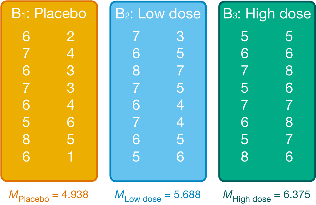
Within each of these three groups, we calculate the overall mean (shown in the figure) and the mean rating of attractive and unattractive faces separately (Table 1).
`summarise()` has regrouped the output.
ℹ Summaries were computed grouped by alcohol and facetype.
ℹ Output is grouped by alcohol.
ℹ Use `summarise(.groups = "drop_last")` to silence this message.
ℹ Use `summarise(.by = c(alcohol, facetype))` for per-operation grouping
(`?dplyr::dplyr_by`) instead.| Alcohol | Type of Face | Mean |
|---|---|---|
| Placebo | Unattractive | 3.500 |
| Placebo | Attractive | 6.375 |
| Low dose | Unattractive | 4.875 |
| Low dose | Attractive | 6.500 |
| High dose | Unattractive | 6.625 |
| High dose | Attractive | 6.125 |
For simple effects of face type at each level of alcohol we’d begin with the placebo and calculate the model sum of squares. The grand mean becomes the mean for all scores in the placebo group and the group means are the mean ratings of attractive and unattractive faces.
We can then apply the model sum of squares equation that we used for the overall model but using the grand mean of the placebo group (4.938) and the mean ratings of unattractive (3.500) and attractive (6.375) faces:
\[ \begin{align} \text{SS}_\text{Face, Placebo} &= \sum_{g = 1}^{k}{n_g\big(\bar{x}_g - \bar{x}_\text{grand}\big)^2} \\ &= 8(3.500 - 4.938)^2 + 8(6.375 - 4.938)^2 \\ &= 33.06 \end{align} \]
The degrees of freedom for this effect are calculated the same way as for any model sum of squares; they are one less than the number of conditions being compared (\(k-1\)), which in this case, where we’re comparing only two conditions, will be 1.
We do the same for the low-dose group. We use the grand mean of the low-dose group (5.688) and the mean ratings of unattractive and attractive faces,
\[ \begin{align} \text{SS}_\text{Face, Low dose} &= \sum_{g = 1}^{k}{n_g\big(\bar{x}_g - \bar{x}_\text{grand}\big)^2} \\ &= 8(4.875 - 5.688)^2 + 8(6.500 - 5.688)^2 \\ &= 10.56 \end{align} \]
The degrees of freedom are again \(k-1\) = 1.
Next, we do the same for the high-dose group. We use the grand mean of the high-dose group (6.375) and the mean ratings of unattractive and attractive faces,
\[ \begin{align} \text{SS}_\text{Face, High dose} &= \sum_{g = 1}^{k}{n_g\big(\bar{x}_g - \bar{x}_\text{grand}\big)^2} \\ &= 8(6.625 - 6.375)^2 + 8(6.125 - 6.375)^2 \\ &= 1. \end{align} \]
Again, the degrees of freedom are 1 (because we’ve compared two groups).
We need to convert these sums of squares to mean squares by dividing by the degrees of freedom but because all of these sums of squares have 1 degree of freedom, the mean squares are the same as the sum of squares. The final stage is to calculate an F-statistic for each simple effect by dividing the mean squares for the model by the residual mean squares. When conducting simple effects we use the residual mean squares for the original model (the residual mean squares for the entire model). In doing so we partition the model sums of squares and keep control of the Type I error rate. For these data, the residual sum of squares was 1.37 (see the book chapter). Therefore, we get:
\[ \begin{align} F_\text{FaceType, Placebo} &= \frac{\text{MS}_\text{Face, Placebo}}{\text{MS}_\text{R}} = \frac{33.06}{1.37} = 24.13 \\ F_\text{FaceType, Low dose} &= \frac{\text{MS}_\text{Face, Low dose}}{\text{MS}_\text{R}} = \frac{10.56}{1.37} = 7.71 \\ F_\text{FaceType, High dose} &= \frac{\text{MS}_\text{Face, High dose}}{\text{MS}_\text{R}} = \frac{1}{1.37} = 0.73 \end{align} \]
These values match those (approximately) in Output 13.3 (p. 747) in the book.
Chapter 14
Please, Sir, can I have some more … ICC?
Field, A. P. (2005). Intraclass correlation. In B. Everitt & D. C. Howell (Eds.), Encyclopedia of Statistics in Behavioral Science (Vol. 2, pp. 948–954). New York: Wiley.
Please, Sir, can I have some more … group mean centring?
We’ll use the cosmetic.csv data to illustrate the two types of centring discussed in the book chapter. Load this file into
cosmetic_tib <- discovr::cosmeticLet’s assume that we want to group_mean centre the variable bdi. Table 2 shows the data for the first 6 cases and Table 3 shows the mean BDI for their corresponding clinics.
The group mean centred values of BDI for each case would be the value of BDI minus the mean BDI in the clinic to which they were assigned. For example, the first case had a BDI score of 32, and was in clinic 5, which had a mean BDI of 18.43. Therefore, their group mean centred BDI would be
\[ \begin{aligned} \text{BDI}_\text{GMC} &= 32 - 18.43 \\ &= 13.57 \end{aligned} \]
Similarly, the second case had a BDI score of 19, and was in clinic 9, which had a mean BDI of 17.04. Therefore, their group mean centred BDI would be
\[ \begin{aligned} \text{BDI}_\text{GMC} &= 19 - 17.04 \\ &= 1.96 \end{aligned} \]
You get the general idea.
| id | post_qol | base_qol | days | clinic | bdi | reason |
|---|---|---|---|---|---|---|
| qx069 | 71 | 56 | 342 | Clinic 5 | 32 | Physical reason |
| v3rjc | 30 | 39 | 349 | Clinic 9 | 19 | Physical reason |
| 33ju1 | 42 | 33 | 208 | Clinic 20 | 7 | Change appearance |
| 5ydxd | 38 | 34 | 242 | Clinic 11 | 30 | Change appearance |
| i6p75 | 69 | 52 | 361 | Clinic 12 | 19 | Change appearance |
| svsuy | 53 | 47 | 41 | Clinic 10 | 24 | Physical reason |
| clinic | mean |
|---|---|
| Clinic 5 | 18.43 |
| Clinic 9 | 17.04 |
| Clinic 20 | 17.64 |
| Clinic 11 | 19.06 |
| Clinic 12 | 17.46 |
| Clinic 10 | 18.18 |
To group-mean centre a variable we use the demean() function from the datawizard package. This function takes the general form:
new_tibble <- demean(x = old_tibble, select = "variable_to_centre", by = "variable_to_group_by")In which we replace new_tibble with a name for our new tibble, old_tibble with the name of our existing data, variable_to_centre with the name of the variable we wish to centre (in this case bdi), and variable_to_group_by with the name of the variable by which we want to group the data (in this case clinic). So, there are three main arguments:
-
x: this specifies the tibble containing the data, in this casecosmetic_tib -
select: this argument allows you to specify the variables to centre (and is used like we use it indescribe_distribution()). In this case we’d specify"bdi"as the variable to centre. We can specify multiple variables by enclosing them inc(). -
by: is to specify the variable representing the groups to use for centring. In this case we’d specify"clinic"because we want to centre BDI by the mean of the clinic to which a person was assigned.
The code below creates a new tibble (cosmetic_gpmc) that includes the results of group mean centring BDI. The first 6 cases are displayed in Table 4. The code creates two new variables:
-
bdi_betweencontains the clinic means and the values match those in Table 3. -
bdi_withincontains the gropup mean centred values ofbdi. Note the values for the first two cases match the hand calculations above.
| id | post_qol | base_qol | days | clinic | bdi | reason | bdi_between | bdi_within |
|---|---|---|---|---|---|---|---|---|
| qx069 | 71 | 56 | 342 | Clinic 5 | 32 | Physical reason | 18.43 | 13.57 |
| v3rjc | 30 | 39 | 349 | Clinic 9 | 19 | Physical reason | 17.04 | 1.96 |
| 33ju1 | 42 | 33 | 208 | Clinic 20 | 7 | Change appearance | 17.64 | -10.64 |
| 5ydxd | 38 | 34 | 242 | Clinic 11 | 30 | Change appearance | 19.06 | 10.94 |
| i6p75 | 69 | 52 | 361 | Clinic 12 | 19 | Change appearance | 17.46 | 1.54 |
| svsuy | 53 | 47 | 41 | Clinic 10 | 24 | Physical reason | 18.18 | 5.82 |
Chapter 15
Please, Sir, can I have some more … sphericity?
Field, A. P. (1998). A bluffer’s guide to sphericity. Newsletter of the Mathematical, Statistical and Computing Section of the British Psychological Society, 6, 13–22.
Chapter 17
Please Sir, can I have some more … matrix algebra?
Calculation of factor score coefficients
The matrix of factor score coefficients (B) and the inverse of the correlation matrix (R−1) for the popularity data are shown below. The matrices R−1 and A can be multiplied by hand to get the matrix B. To get the same degree of accuracy as
\[ \begin{align} B &= R^{- 1}A \\ &= \begin{pmatrix} 4.76 & -7.46 & 3.91 & -2.35 & 2.42 & -0.49 \\ -7.46 & 18.49 & -12.42 & 5.45 & -5.54 & 1.22 \\ 3.91 & -12.42 & 10.07 & - 3.65 & 3.79 & -0.96 \\ -2.35 & 5.45 & -3.65 & 2.97 & -2.16 & 0.02 \\ 2.42 & -5.54 & 3.79 & - 2.16 & 2.98 & -0.56 \\ -0.49 & 1.22 & -0.96 & 0.02 & -0.56 & 1.27 \\ \end{pmatrix}\begin{pmatrix} 0.87 & 0.01 \\ 0.96 & -0.03 \\ 0.92 & 0.04 \\ 0.00 & 0.82 \\ -0.10 & 0.75 \\ 0.09 & 0.70 \\ \end{pmatrix}\\ &=\begin{pmatrix} 0.343 & 0.006 \\ 0.376 & -0.020 \\ 0.362 & 0.020 \\ 0.000 & 0.473 \\ -0.037 & 0.437 \\ 0.039 & 0.405 \\ \end{pmatrix} \end{align} \]
Column 1 of matrix B
To get the first element of the first column of matrix B, you need to multiply each element in the first column of matrix A with the correspondingly placed element in the first row of matrix R−1. Add these six products together to get the final value of the first element. To get the second element of the first column of matrix B, you need to multiply each element in the first column of matrix A with the correspondingly placed element in the second row of matrix R−1. Add these six products together to get the final value … and so on:
\[ \begin{align} B_{11} &= (4.76 \times 0.87) + (-7.46 \times 0.96) + (3.91 \times 0.92 ) + (-2.35 \times -0.00) + (2.42 \times -0.10) + (-0.49 \times 0.09)\\ &= 0.343\\ B_{21} &= (-7.46 \times 0.87) + \ (18.49 \times 0.96) + (-12.42 \times 0.92) + (5.45 \times -0.00) + (-5.54 \times -0.10) + ( 1.22 \times 0.09)\\ &= 0.376\\ B_{31} &= (3.91 \times 0.87) + (-12.42 \times 0.96) + (10.07 \times 0.92) + (-3.65 \times -0.00) + (3.70 \times - 0.10 ) + (-0.96 \times 0.09 )\\ &= 0.362\\ B_{41} &= (-2.35 \times 0.87) + ( 5.45\ \times 0.96) + (-3.65 \times 0.92 ) + ( 2.97 \times -0.00 ) + (-2.16 \times -0.10 ) + (0.02\ \times \ 0.09)\\ &= 0.000\\ B_{51} &= (2.42 \times 0.87) + (-5.54\ \times 0.96) + (3.79 \times 0.92 ) + (-2.16 \times -0.00 ) + (2.98 \times -0.10 ) + (- 0.56\ \times 0.09)\\ &= -0.037\\ B_{61} &= (-0.49 \times 0.87) + (1.22 \times 0.96) + (-0.96 \times 0.92 ) + ( 0.02 \times -0.00) + (-0.56 \times -0.10 ) + (1.27 \times 0.09)\\ &= 0.039 \end{align} \]
Column 2 of matrix B
To get the first element of the second column of matrix B, you need to multiply each element in the second column of matrix A with the correspondingly placed element in the first row of matrix R−1. Add these six products together to get the final value. To get the second element of the second column of matrix B, you need to multiply each with the correspondingly placed element in the second row of matrix R−1. Add these six products together to get the final value … and so on:
\[ \begin{align} B_{12} &= (4.76 \times 0.01) + (-7.46 \times -0.03) + (3.91 \times 0.04) + (-2.35 \times 0.82) + (2.42 \times 0.75) + (-0.49 \times 0.70)\\ &= 0.006\\ B_{22} &= (-7.46 \times 0.01) + \ (18.49 \times -0.03) + (-12.42 \times0.04) + (5.45 \times 0.82) + (-5.54 \times 0.75) + (1.22 \times 0.70)\\ &=-0.020\\ B_{32} &= (3.91 \times 0.01) + (-12.42 \times -0.03) + (10.07 \times 0.04) + (-3.65 \times 0.82) + (3.70 \times 0.75) + (-0.96 \times 0.70)\\ &= 0.020\\ B_{42} &= (-2.35 \times 0.01) + ( 5.45\ \times -0.03) + (-3.65 \times 0.04) + ( 2.97 \times 0.82) + (-2.16 \times 0.75) + (0.02\ \times \ 0.70)\\ &= 0.473\\ B_{52} &= (2.42 \times 0.01) + (-5.54\ \times -0.03) + (3.79 \times 0.04) + (-2.16 \times 0.82) + (2.98 \times 0.75) + (- 0.56\ \times 0.70)\\ &= 0.473\\ B_{62} &= (-0.49 \times 0.01) + (1.22 \times -0.03) + (-0.96 \times 0.04) + ( 0.02 \times 0.82) + (-0.56 \times 0.75) + (1.27 \times 0.70)\\ &= 0.405 \end{align} \]
Factor scores
The pattern of the loadings is the same for the factor score coefficients: that is, the first three variables have high loadings for the first factor and low loadings for the second, whereas the pattern is reversed for the last three variables. The difference is only in the actual value of the weightings, which are smaller because the correlations between variables are now accounted for. These factor score used to replace the b-values in the equation for the factor:
\[ \begin{align} \text{Sociability}_i &= 0.343\text{Talk 1}_i + 0.376\text{Social skills}_i + 0.362\text{Interest}_i + 0.00\text{Talk 2}_i - 0.037\text{Selfish}_i + 0.039\text{Liar}_i\\ &= (0.343 \times 4) + (0.376 \times 9) + (0.362 \times 8) + (0.00 \times 6) - (0.037\times 8) + (0.039\times 6)\\ &= 7.59\\ \text{Consideration}_i &= 0.006\text{Talk 1}_i - 0.020\text{Social skills}_i + 0.020\text{Interest}_i + 0.473\text{Talk 2}_i + 0.437\text{Selfish}_i + 0.405\text{Liar}_i\\ &= (0.006 \times 4) - (0.020 \times 9) + (0.020 \times 8) + (0.473 \times 6) + (0.437 \times 8) + (0.405 \times 6)\\ &= 8.768 \end{align} \]
In this case, we use the same participant scores on each variable as were used in the chapter. The resulting scores are much more similar than when the factor loadings were used as weights because the different variances among the six variables have now been controlled for. The fact that the values are very similar reflects the fact that this person not only scores highly on variables relating to sociability, but is also inconsiderate (i.e., they score equally highly on both factors).
Please, Sir, can I have some more … questionnaires?
As a rule of thumb, never to attempt to design a questionnaire! A questionnaire is very easy to design, but a good questionnaire is virtually impossible to design. The point is that it takes a long time to construct a questionnaire, with no guarantees that the end result will be of any use to anyone. A good questionnaire must have three things: discrimination, reliability and validity.
Discrimination
Discrimination is really an issue of item selection. Discrimination simply means that people with different scores on a questionnaire differ in the construct of interest to you. For example, a questionnaire measuring social phobia should discriminate between people with social phobia and people without it (i.e., people in the different groups should score differently). There are three corollaries to consider:
- People with the same score should be equal to each other along the measured construct.
- People with different scores should be different to each other along the measured construct.
- The degree of difference between people is proportional to the difference in scores.
This is all pretty self-evident really, so what’s the fuss about? Well, let’s take a really simple example of a three-item questionnaire measuring sociability. Imagine we administered this questionnaire to two people: Jane and Katie. Their responses are shown below.
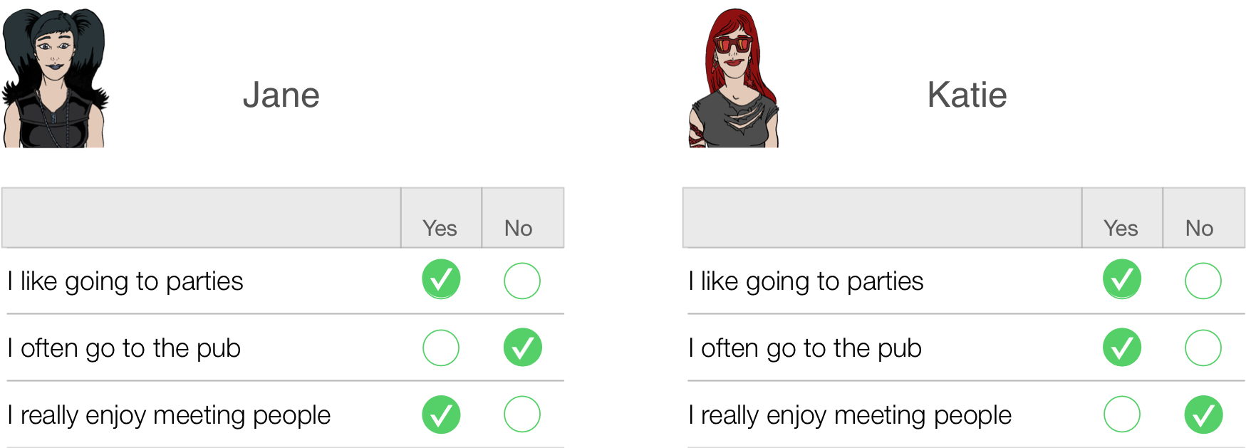
Jane responded yes to items 1 and 3 but no to item 2. If we score a yes with the value 1 and a no with a 0, then we can calculate a total score of 2. Katie, on the other hand, answers yes to items 1 and 2 but no to item 3. Using the same scoring system her score is also 2. Therefore, numerically you have identical answers (i.e. both Jane and Katie score 2 on this questionnaire); therefore, these two people should be comparable in their sociability — are they?
The answer is: not necessarily. It seems that Katie likes to go to parties and the pub but doesn’t enjoy meeting people in general, whereas Jane enjoys parties and meeting people but doesn’t enjoy the pub. It seems that Katie likes social situations involving alcohol (e.g. the pub and parties) but Jane likes socializing in general, but doesn’t like pubs — perhaps because there are more strangers there than at parties. In many ways, therefore, these people are very different because our questions are contaminated by other factors (i.e. attitudes to alcohol or different social environments). A good questionnaire should be designed such that people with identical numerical scores are identical in the construct being measured — and that’s not as easy to achieve as you might think!
A second related point is score differences. Imagine you take scores on the Spider Phobia Questionnaire. Imagine you have three participants who do the questionnaire and get the following scores: Andy scores 30 on the SPQ (very spider phobic), Graham scores 15 (moderately phobic) and Dan scores 10 (not very phobic at all). Does this mean that Dan and Graham are more similar in their spider phobia than Graham and Andy? In theory this should be the case because Graham’s score is more similar to Dan’s (difference = 5) than it is to Andy’s (difference = 15). In addition, is it the case that Andy is three times more phobic of spiders than Dan is? Is he twice as phobic as Graham? Again, his scores suggest that he should be. The point is that you can’t guarantee in advance that differences in score are going to be comparable, yet a questionnaire needs to be constructed such that the difference in score is proportional to the difference between people.
Validity
Items on your questionnaire must measure something, and a good questionnaire measures what you designed it to measure (this is called validity). Validity basically means ‘measuring what you think you’re measuring’. So, an anxiety measure that actually measures assertiveness is not valid; however, a materialism scale that does actually measure materialism is valid. Validity is a difficult thing to assess and it can take several forms:
-
Content validity. Items on a questionnaire must relate to the construct being measured. For example, a questionnaire measuring intrusive thoughts is pretty useless if it contains items relating to statistical ability. Content validity is really how representative your questions are — the sampling adequacy of items. This is achieved when items are first selected: don’t include items that are blatantly very similar to other items, and ensure that questions cover the full range of the construct.
- Criterion validity. This is basically whether the questionnaire is measuring what it claims to measure. In an ideal world, you could assess this by relating scores on each item to real-world observations (e.g., comparing scores on sociability items with the number of times a person actually goes out to socialize). This is often impractical and so there are other techniques such as (a) using the questionnaire in a variety of situations and seeing how predictive it is; (b) seeing how well it correlates with other known measures of your construct (i.e., sociable people might be expected to score highly on extroversion scales); and (c) using statistical techniques such as the Item Validity Index.
- Factorial validity. This validity basically refers to whether the factor structure of the questionnaire makes intuitive sense. As such, factorial validity is assessed through factor analysis. When you have your final set of items you can conduct a factor analysison the data (see the book). Factor analysis takes your correlated questions and recodes them into uncorrelated, underlying variables called factors (an example might be recoding the variables height, chest size, shoulder width and weight into an underlying variable called ‘build’). As another example, to assess success in a course we might measure attentiveness in seminars, the amount of notes taken in seminars, and the number of questions asked during seminars — all of these variables may relate to an underlying trait such as ‘motivation to succeed’. Factor analysis produces a table of items and their correlation, or loading, with each factor. A factor is composed of items that correlate highly with it. Factorial validity can be seen from whether the items tied on to factors make intuitive sense or not. Basically, if your items cluster into meaningful groups then you can infer factorial validity.
Validity is a necessary but not sufficient condition of a questionnaire.
Reliability
A questionnaire must be not only valid, but also reliable. Reliability is basically the ability of the questionnaire to produce the same results under the same conditions. To be reliable the questionnaire must first be valid. Clearly the easiest way to assess reliability is to test the same group of people twice: if the questionnaire is reliable you’d expect each person’s scores to be the same at both points in time. So, scores on the questionnaire should correlate perfectly (or very nearly!). However, in reality, if we did test the same people twice then we’d expect some practice effects and confounding effects (people might remember their responses from last time). Also this method is not very useful for questionnaires purporting to measure something that we would expect to change (such as depressed mood or anxiety). These problems can be overcome using the alternate form method in which two comparable questionnaires are devised and compared. Needless to say, this is a rather time-consuming way to ensure reliability and fortunately thereare statistical methods to make life much easier.
The simplest statistical technique is the split-half method. This method randomly splits the questionnaire items into two groups. A score for each subject is then calculated based on each half of the scale. If a scale is very reliable we’d expect a person’s score to be the same on one half of the scale as on the other, and so the two halves should correlate perfectly. The correlation between the two halves is the statistic computed in the split-half method, large correlations being a sign of reliability.[^1] The problem with this method is that there are a number of ways in which a set of data can be split into two and so the results might be a result of the way in which the data were split. To overcome this problem, Cronbach suggested splitting the data in two in every conceivable way and computing the correlation coefficient for each split. The average of these values is known as Cronbach’s alpha, which is the most common measure of scale reliability. As a rough guide, a value of .8 is seen as an acceptable value for Cronbach’s alpha; values substantially lower indicate an unreliable scale (see the book for more detail).
How to design your questionnaire
Step 1: Choose a construct
First you need to decide on what you would like to measure. Once you have done this, use PsychLit and the Web of Knowledge to do a basic search for some information on this topic. I don’t expect you to search through reams of material, but just get some basic background on the construct you’re testing and how it might relate to psychologically important things. For example, if you looked at empathy, this is seen as an important component of Carl Roger’s client-centred therapy; therefore, having the personality trait of empathy might be useful if you were to become a Rogerian therapist. It follows then that having a questionnaire to measure this trait might be useful for selection purposes on Rogerian therapy training courses. So, basically you need to set some kind of context as to why the construct is important — this information will form the basis of your introduction.
Step 2: Decide on a response scale
A fundamental issue is how you want respondents to answer questions. You could choose to have:
- Yes/no or yes/no/don’t know scales. This forces people to give one answer or another even though they might feel that they are neither a yes nor no. Also, imagine you were measuring intrusive thoughts and you had an item ‘I think about killing children’. Chances are everyone would respond no to that statement (even if they did have those thoughts) because it is a very undesirable thing to admit. Therefore, all this item is doing is subtracting a value from everybody’s score — it tells you nothing meaningful, it is just noise in the data. This scenario can also occur when you have a rating scale with a don’t know response (because people just cannot make up their minds and opt for the neutral response). This is why it is sometimes nice to have questionnaires with a neutral point to help you identify which things people really have no feeling about. Without this midpoint you are simply making people go one way or the other, which is comparable to balancing a coin on its edge and seeing which side up it lands when it falls. Basically, when forced, 50% will choose one option while 50% will choose the opposite — this is just noise in your data.
- Likert scale. This is the standard agree–disagree ordinal categories response. It comes in many forms:
- 3-point: agree ⇒ neither agree nor disagree ⇒ disagree
- 5-point: agree ⇒ midpoint ⇒ neither agree nor disagree ⇒ midpoint ⇒ disagree
- 7-Point: agree ⇒ 2 points ⇒ neither agree nor disagree ⇒ 2 points ⇒ disagree
Questions should encourage respondents to use all points of the scale. So, ideally the statistical distribution of responses to a single item should be normal with a mean that lies at the centre of the scale (so on a 5-point Likert scale the mean on a given question should be 3). The range of scores should also cover all possible responses.
Step 3: Generate your items
Once you’ve found a construct to measure and decided on the type of response scale you’re going to use, the next task is to generate items. I want you to restrict your questionnaire to around 30 items (20 minimum). The best way to generate items is to ‘brainstorm’ a small sample of people. This involves getting people to list as many facets of your construct as possible. For example, if you devised a questionnaire on exam anxiety, you might ask a number of students (20 or so) from a variety of courses (arts and science), years (first, second and final) and even institutions (friends at other universities) to list (on a piece of paper) as many things about exams as possible that make them anxious. It is good if you can include people within this sample that you think might be at the extremes of your construct (e.g., select a few people who get very anxious about exams and some who are very calm). This enables you to get items that span the entire spectrum of the construct that you want to measure.
This will give you a pool of items to inspire questions. Rephrase your sample’s suggestions in a way that fits the rating scale you’ve chosen and then eliminate any questions that are basically the same. You should hopefully begin with a pool of say 50–60 questions that you can reduce to about 30 by eliminating obviously similar questions.
## Things to consider
- Wording of questions. The way in which questions are phrased can bias the answers that people give; For example, (Gaskell et al., 1993) report several studies in which subtle changes in the wording of survey questions can radically affect people’s responses. Gaskell et al.’s article is a very readable and useful summary of this work and their conclusions might be useful to you when thinking about how to phrase your questions.
- Response bias. This is the tendency of respondents to give the same answer to every question. Try to reverse-phrase a few items to avoid response bias (and remember to score these items in reverse when you enter the data into ).
Step 4: Collect the data
Once you’ve written your questions, randomize their order and produce your questionnaire. This is the questionnaire that you’re going to test. Administer it to as many people as possible (one benefit of making these questionnaires short is that it minimizes the time taken to complete them!). You should aim for 300+ respondents, but the more you get, the better your analysis (which is why I suggest working in slightly bigger groups to make data collection easier).
Step 5: Analysis
Enter the data into
What we’re trying to do with this analysis is to first eliminate any items on the questionnaire that aren’t useful. So, we’re trying to reduce our 30 items further before we run our factor analysis. We can do this by looking at descriptive statistics and also correlations between questions.
Descriptive statistics. The first thing to look at is the statistical distribution of item scores. This alone will enable you to throw out many redundant items. Therefore, the first thing to do when piloting a questionnaire is look at descriptive statistics on the questionnaire items. This is easily done in
- Range. Any item that has a limited range (all the points of the scale have not been used).
- Skew. I mentioned above that ideally each question should elicit a normally distributed set of responses across subjects (each item’s mean should be at the centre of the scale and there should be no skew). To check for items that produce skewed data, look for the skewness and SE skew in your output. Skew doesn’t affect factor analysis per se, it’s more that highly skewed questions are not eliciting a range of responses.
Correlations. All of your items should intercorrelate at a reasonable level if they are measuring aspects of the same thing. If any items have low correlations (< .2) with many other items then exclude them. You can get a table of correlations: from
Factor analysis: When you’ve eliminated any items that have distributional problems or do not correlate with each other, then run your factor analysis on the remaining items and try to interpret the resulting factor structure. The book chapter details the process of factor analysis. What you should do is examine the factor structure and decide:
- Which factors to retain.
- Which items load on to those factors.
- What your factors represent.
If there are any items that don’t load highly on to any factors, they should be eliminated from future versions of the questionnaire (for our purposes you need only state that they are not useful items as you won’t have time to revise and retest your questionnaires!)
Step 6: Assess the questionnaire
Having looked at the factor structure, you need to check the reliability of your items and the questionnaire as a whole. You should run a reliability analysis on the questionnaire. This is explained in Chapter 18 of the book. There are two things to look at: (1) the Item Reliability Index (IRI), which is the correlation between the score on the item and the score on the test as a whole multiplied by the standard deviation of that item (called the corrected item–total correlation in
The end?
You should conclude by describing your factor structure and the reliability of the scale. Also say whether there are items that you would drop in a future questionnaire. In an ideal world we’d then generate new items to add to the retained items and start the whole process again!