Labcoat Leni solutions Chapter 18

World wide addiction?
Load the data
To load the data from the CSV file (assuming you have set up a project folder as suggested in the book) and set the factor and its levels:
ias_tib <- readr::read_csv("../data/nichols_2004.csv") %>%
  dplyr::mutate(
    gender = forcats::as_factor(gender),
  )
Alternative, load the data directly from the discovr package:
ias_tib <- discovr::nichols_2004
Let’s also create a version of the data that only contains the items (i.e. removes the participant ID and gender):
ias_items_tib <- ias_tib %>%
  dplyr::select(-c(participant_code, gender))
Descriptive statistics
To get the descriptive statistics (we’ll look only at means and standard deviations) execute the code below, which transforms the data from messy to tidy, renames the items (not necessary but prettier), groups by item, computes the descriptive statistics, then sorts the items by the value of the mean (in ascending order so the low means come first) and prints using kable() rounding to 2 decimal places.
ias_tib %>%
  tidyr::pivot_longer(
    cols = ias1:ias36,
    names_to = "Item",
    values_to = "Response"
  ) %>%
  dplyr::mutate(
    Item = gsub("ias", "IAS ", Item)
  ) %>%
  dplyr::group_by(Item) %>%
  dplyr::summarize(
    Mean = mean(Response),
    SD = sd(Response)
  ) %>%
  dplyr::arrange(Mean) %>%
  knitr::kable(digits = 2)
| Item | Mean | SD |
|---|---|---|
| IAS 34 | 1.11 | 0.34 |
| IAS 23 | 1.14 | 0.43 |
| IAS 6 | 1.22 | 0.57 |
| IAS 29 | 1.23 | 0.57 |
| IAS 15 | 1.23 | 0.52 |
| IAS 28 | 1.24 | 0.56 |
| IAS 26 | 1.25 | 0.57 |
| IAS 22 | 1.25 | 0.66 |
| IAS 36 | 1.27 | 0.58 |
| IAS 16 | 1.30 | 0.69 |
| IAS 17 | 1.31 | 0.68 |
| IAS 20 | 1.32 | 0.64 |
| IAS 14 | 1.33 | 0.64 |
| IAS 18 | 1.33 | 0.68 |
| IAS 33 | 1.35 | 0.75 |
| IAS 10 | 1.36 | 0.70 |
| IAS 25 | 1.39 | 0.69 |
| IAS 7 | 1.41 | 0.80 |
| IAS 11 | 1.48 | 0.76 |
| IAS 1 | 1.49 | 0.82 |
| IAS 35 | 1.50 | 0.84 |
| IAS 30 | 1.51 | 0.80 |
| IAS 5 | 1.51 | 0.85 |
| IAS 32 | 1.54 | 0.90 |
| IAS 21 | 1.58 | 0.96 |
| IAS 2 | 1.59 | 0.93 |
| IAS 9 | 1.66 | 0.96 |
| IAS 12 | 1.71 | 0.86 |
| IAS 24 | 1.89 | 0.96 |
| IAS 27 | 1.91 | 0.98 |
| IAS 4 | 2.01 | 1.07 |
| IAS 13 | 2.03 | 1.12 |
| IAS 19 | 2.03 | 0.95 |
| IAS 8 | 2.09 | 1.13 |
| IAS 31 | 2.27 | 1.03 |
| IAS 3 | 2.68 | 1.07 |
The table of means and standard deviations shows that the items with the lowest values are IAS 23 (I see my friends less often because of the time that I spend on the Internet) and IAS 34 (When I use the Internet, I experience a buzz or a high).
Rather than obtain a table of correlations (which will be very large), we’ll use cor.plot() to visualise the relationships between the items. (Remember to use the tibble that contains only the items of the questionnaire.)
psych::cor.plot(ias_items_tib, upper = FALSE)
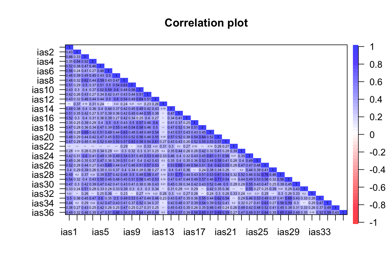
We know that the authors eliminated three items for having low correlations. Remember that cor.plot() colours the cells according to the strength of correlation: the weker the correlation the paler the shading of the cell with zero correlations having no shading at all (i.e. white). So, we’re looking for variables that have a lot of cells with very pale shading. The three items that stand out are IAS 13 (I have felt a persistent desire to cut down or control my use of the internet), IAS 22 (I have neglected things which are important and need doing), and IAS-32 (I find myself thinking/longing about when I will go on the internet again.). As such these variables will also be excluded from the analysis.
Drop unwanted items
Based on the above, we want to remove items IAS 13, IAS 22, IAS 23, IAS 32, IAS 34. We can do this by recreating ias_items_tib without these items:
ias_items_tib <- ias_items_tib %>%
  dplyr::select(-c(ias13, ias22, ias23, ias32, ias34))
Initial checks
To get Bartlett’s test and the KMO execute
cor(ias_items_tib) %>%
  psych::cortest.bartlett(., n = 2571)
## $chisq
## [1] 55672.37
##
## $p.value
## [1] 0
##
## $df
## [1] 465
psych::KMO(ias_items_tib)
## Kaiser-Meyer-Olkin factor adequacy
## Call: psych::KMO(r = ias_items_tib)
## Overall MSA =  0.94
## MSA for each item =
##  ias1  ias2  ias3  ias4  ias5  ias6  ias7  ias8  ias9 ias10 ias11 ias12 ias14
##  0.95  0.90  0.94  0.92  0.95  0.92  0.92  0.95  0.96  0.94  0.95  0.96  0.94
## ias15 ias16 ias17 ias18 ias19 ias20 ias21 ias24 ias25 ias26 ias27 ias28 ias29
##  0.92  0.94  0.96  0.96  0.97  0.96  0.96  0.95  0.95  0.94  0.93  0.92  0.94
## ias30 ias31 ias33 ias35 ias36
##  0.95  0.89  0.93  0.92  0.95
Sample size: The KMO statistic (Overall MSA) is 0.94, which is well above the minimum criterion of 0.5 and falls into the range of marvellous. The KMO values for individual variables range from 0.89 to 0.97. All values are, therefore, well above 0.5, which is good news.
Bartlett’s test: This test is significant, $ \chi^2 = $(465) = 5.567237^{4}, p = 0, indicating that the correlations within the R-matrix are sufficiently different from zero to warrant PCA.
Parallel analysis
The authors didn’t use parallel analysis, but let’s do it anyway.
psych::fa.parallel(ias_items_tib, fa = "pc")
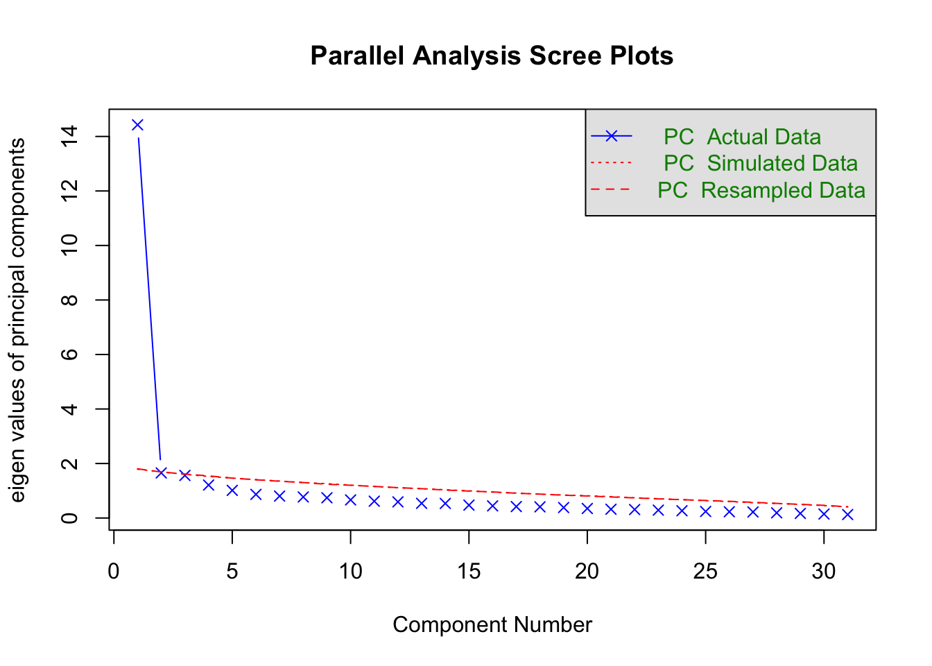
## Parallel analysis suggests that the number of factors = NA and the number of components = 1
The parallel analysis suggests that a single component underlies the items, which is consistent with what the authors conclude based on the scree plot (see below).
Principal components analysis
To do the principal component analysis execute the code below. Because we are retaining only one component we don’t need to specify a rotation method.
ias_fa <- psych::pca(ias_items_tib,
                    nfactors = 1)
ias_fa
## Principal Components Analysis
## Call: principal(r = r, nfactors = nfactors, residuals = residuals,
##     rotate = rotate, n.obs = n.obs, covar = covar, scores = scores,
##     missing = missing, impute = impute, oblique.scores = oblique.scores,
##     method = method, use = use, cor = cor, correct = 0.5, weight = NULL)
## Standardized loadings (pattern matrix) based upon correlation matrix
##        PC1   h2   u2 com
## ias1  0.70 0.49 0.51   1
## ias2  0.48 0.23 0.77   1
## ias3  0.68 0.46 0.54   1
## ias4  0.56 0.31 0.69   1
## ias5  0.69 0.48 0.52   1
## ias6  0.67 0.45 0.55   1
## ias7  0.70 0.49 0.51   1
## ias8  0.74 0.55 0.45   1
## ias9  0.72 0.52 0.48   1
## ias10 0.73 0.53 0.47   1
## ias11 0.67 0.45 0.55   1
## ias12 0.72 0.52 0.48   1
## ias14 0.67 0.44 0.56   1
## ias15 0.68 0.47 0.53   1
## ias16 0.55 0.30 0.70   1
## ias17 0.65 0.43 0.57   1
## ias18 0.71 0.51 0.49   1
## ias19 0.75 0.56 0.44   1
## ias20 0.79 0.62 0.38   1
## ias21 0.74 0.55 0.45   1
## ias24 0.72 0.52 0.48   1
## ias25 0.66 0.44 0.56   1
## ias26 0.77 0.60 0.40   1
## ias27 0.53 0.28 0.72   1
## ias28 0.74 0.54 0.46   1
## ias29 0.76 0.57 0.43   1
## ias30 0.64 0.41 0.59   1
## ias31 0.50 0.25 0.75   1
## ias33 0.71 0.51 0.49   1
## ias35 0.56 0.31 0.69   1
## ias36 0.80 0.64 0.36   1
##
##                  PC1
## SS loadings    14.43
## Proportion Var  0.47
##
## Mean item complexity =  1
## Test of the hypothesis that 1 component is sufficient.
##
## The root mean square of the residuals (RMSR) is  0.07
##  with the empirical chi square  912.89  with prob <  3e-36
##
## Fit based upon off diagonal values = 0.98
We can print the loadings in a nice table as:
parameters::model_parameters(ias_fa) %>%
  knitr::kable(digits = 2)
| Variable | PC1 | Complexity | Uniqueness |
|---|---|---|---|
| ias1 | 0.70 | 1 | 0.51 |
| ias2 | 0.48 | 1 | 0.77 |
| ias3 | 0.68 | 1 | 0.54 |
| ias4 | 0.56 | 1 | 0.69 |
| ias5 | 0.69 | 1 | 0.52 |
| ias6 | 0.67 | 1 | 0.55 |
| ias7 | 0.70 | 1 | 0.51 |
| ias8 | 0.74 | 1 | 0.45 |
| ias9 | 0.72 | 1 | 0.48 |
| ias10 | 0.73 | 1 | 0.47 |
| ias11 | 0.67 | 1 | 0.55 |
| ias12 | 0.72 | 1 | 0.48 |
| ias14 | 0.67 | 1 | 0.56 |
| ias15 | 0.68 | 1 | 0.53 |
| ias16 | 0.55 | 1 | 0.70 |
| ias17 | 0.65 | 1 | 0.57 |
| ias18 | 0.71 | 1 | 0.49 |
| ias19 | 0.75 | 1 | 0.44 |
| ias20 | 0.79 | 1 | 0.38 |
| ias21 | 0.74 | 1 | 0.45 |
| ias24 | 0.72 | 1 | 0.48 |
| ias25 | 0.66 | 1 | 0.56 |
| ias26 | 0.77 | 1 | 0.40 |
| ias27 | 0.53 | 1 | 0.72 |
| ias28 | 0.74 | 1 | 0.46 |
| ias29 | 0.76 | 1 | 0.43 |
| ias30 | 0.64 | 1 | 0.59 |
| ias31 | 0.50 | 1 | 0.75 |
| ias33 | 0.71 | 1 | 0.49 |
| ias35 | 0.56 | 1 | 0.69 |
| ias36 | 0.80 | 1 | 0.36 |
The table of factor loadings shows that all items have a high loading on the one component we extracted.
The authors reported their analysis as follows (p. 382):
We conducted principal-components analyses on the log transformed scores of the IAS (see above). On the basis of the scree test (Cattell, 1978) and the percentage of variance accounted for by each factor, we judged a one-factor solution to be most appropriate. This component accounted for a total of 46.50% of the variance. A value for loadings of .30 (Floyd & Widaman, 1995) was used as a cut-off for items that did not relate to a component.
All 31 items loaded on this component, which was interpreted to represent aspects of a general factor relating to Internet addiction reflecting the negative consequences of excessive Internet use.