Labcoat Leni solutions Chapter 11

This document contains abridged sections from Discovering Statistics Using R and RStudio by Andy Field so there are some copyright considerations. You can use this material for teaching and non-profit activities but please do not meddle with it or claim it as your own work. See the full license terms at the bottom of the page.
Scraping the barrel?
Load the data
To load the data from the CSV file (assuming you have set up a project folder as suggested in the book) and set the factor and its levels:
phallus_tib <- readr::read_csv("../data/gallup_2003.csv") %>%
  dplyr::mutate(
    phallus = forcats::as_factor(phallus) %>% forcats::fct_relevel(., "No Coronal Ridge", "Minimal Coronal Ridge", "Coronal Ridge")
  )
Alternative, load the data directly from the discovr package:
phallus_tib <- discovr::gallup_2003
Plot the data
Let’s do the plot first. There are two variables: phallus (the predictor variable that has three levels: no ridge, minimal ridge and normal ridge) and displace (the outcome variable, the percentage of sperm displaced). The plot should therefore plot phallus on the x-axis and displace on the y-axis. We can get an error bar plot as follows:
ggplot2::ggplot(phallus_tib, aes(phallus, displace)) +
  stat_summary(fun.data = "mean_cl_boot", colour = "#5c97bf") +
  coord_cartesian(ylim = c(0, 100)) +
  scale_y_continuous(breaks = seq(0, 100, 10)) +
  labs(x = "Phallus shape", y = "Percentage of sperm displaced") +
  theme_minimal()
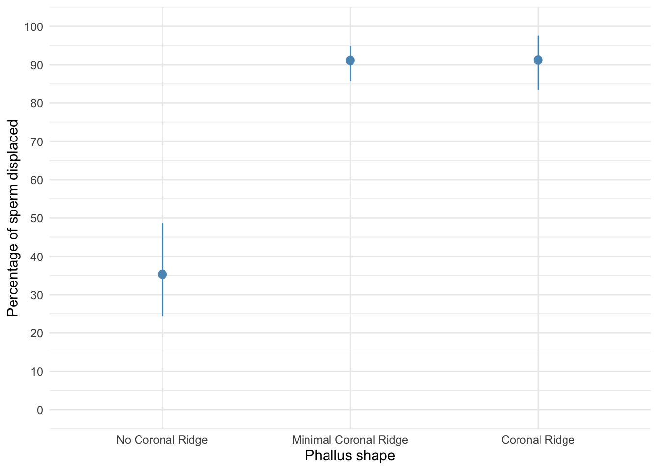
The plot shows that having a coronal ridge results in more sperm displacement than not having one. The size of ridge made very little difference:
Fit the model
To test our hypotheses we need to first enter the following codes for the contrasts:
| Group | No ridge vs. ridge | Minimal vs. coronal |
|---|---|---|
| No Ridge | -2/3 | 0 |
| Minimal ridge | 1/3 | -1/2 |
| Coronal ridge | 1/3 | 1/2 |
Contrast 1 tests hypothesis 1: that having a bell-end will displace more sperm than not. To test this we compare the two conditions with a ridge against the control condition (no ridge). So we compare chunk 1 (no ridge) to chunk 2 (minimal ridge, coronal ridge). The numbers assigned to the groups are the number of groups in the opposite chunk divided by the number of groups that have non-zero codes, and we randomly assigned one chunk to be a negative value (the codes 2/3, −1/3, −1/3 would work fine as well).
Contrast 2 tests hypothesis 2: the phallus with the larger coronal ridge will displace more sperm than the phallus with the minimal coronal ridge. First we get rid of the control phallus by assigning a code of 0; next we compare chunk 1 (minimal ridge) to chunk 2 (coronal ridge). The numbers assigned to the groups are the number of groups in the opposite chunk divided by the number of groups that have non-zero codes, and then we randomly assigned one chunk to be a negative value (the codes 0, 1/2, −1/2 would work fine as well).
We set these contrasts for the variable phallus as follows:
ridge_vs_none <- c(-2/3, 1/3, 1/3)
minimal_vs_coronal <- c(0, -1/2, 1/2)

contrasts(phallus_tib$phallus) <- cbind(ridge_vs_none, minimal_vs_coronal)
contrasts(phallus_tib$phallus) # check the contrasts are set correctly
##                       ridge_vs_none minimal_vs_coronal
## No Coronal Ridge         -0.6666667                0.0
## Minimal Coronal Ridge     0.3333333               -0.5
## Coronal Ridge             0.3333333                0.5
Next we fit the model using this code:
phallus_lm <- lm(displace ~ phallus, data = phallus_tib, na.action = na.exclude)

anova(phallus_lm) %>%
  parameters::parameters(., omega_squared = "raw") %>%
  knitr::kable(digits = 3)
| Parameter | Sum_Squares | df | Mean_Square | F | p | Omega_Sq_partial |
|---|---|---|---|---|---|---|
| phallus | 10397.657 | 2 | 5198.829 | 41.559 | 0 | 0.844 |
| Residuals | 1501.128 | 12 | 125.094 | NA | NA | NA |
The output tells us that there was a significant effect of the type of phallus, F(2, 12) = 41.56, p < .001. (This is exactly the same result as reported in the paper on page 280.). View the parameters using:
broom::tidy(phallus_lm, conf.int = TRUE) %>%
  knitr::kable(digits = 3)
| term | estimate | std.error | statistic | p.value | conf.low | conf.high |
|---|---|---|---|---|---|---|
| (Intercept) | 72.549 | 2.888 | 25.122 | 0.000 | 66.257 | 78.841 |
| phallusridge_vs_none | 55.851 | 6.126 | 9.117 | 0.000 | 42.503 | 69.198 |
| phallusminimal_vs_coronal | 0.114 | 7.074 | 0.016 | 0.987 | -15.299 | 15.526 |
The output shows that hypothesis 1 is supported (phallusridge_vs_none): having some kind of ridge led to greater sperm displacement than not having a ridge, b = 55.85 [42.50, 69.20], t(12) = 9.12, p < .001. Hypothesis 2 is not supported (phallusminimal_vs_coronal): the amount of sperm displaced by the normal coronal ridge was not significantly different from the amount displaced by a minimal coronal ridge, b = 0.11 [$-15.30$, 15.53], t(12) = 0.02, p = .987.
Check model diagnostics
We can get some basic diagnostic plots as follows:
library(ggfortify) # remember to load this package
ggplot2::autoplot(phallus_lm,
                  which = c(1, 3, 2, 4),
                  colour = "#5c97bf",
                  smooth.colour = "#ef4836",
                  alpha = 0.5,
                  size = 1) +
  theme_minimal()
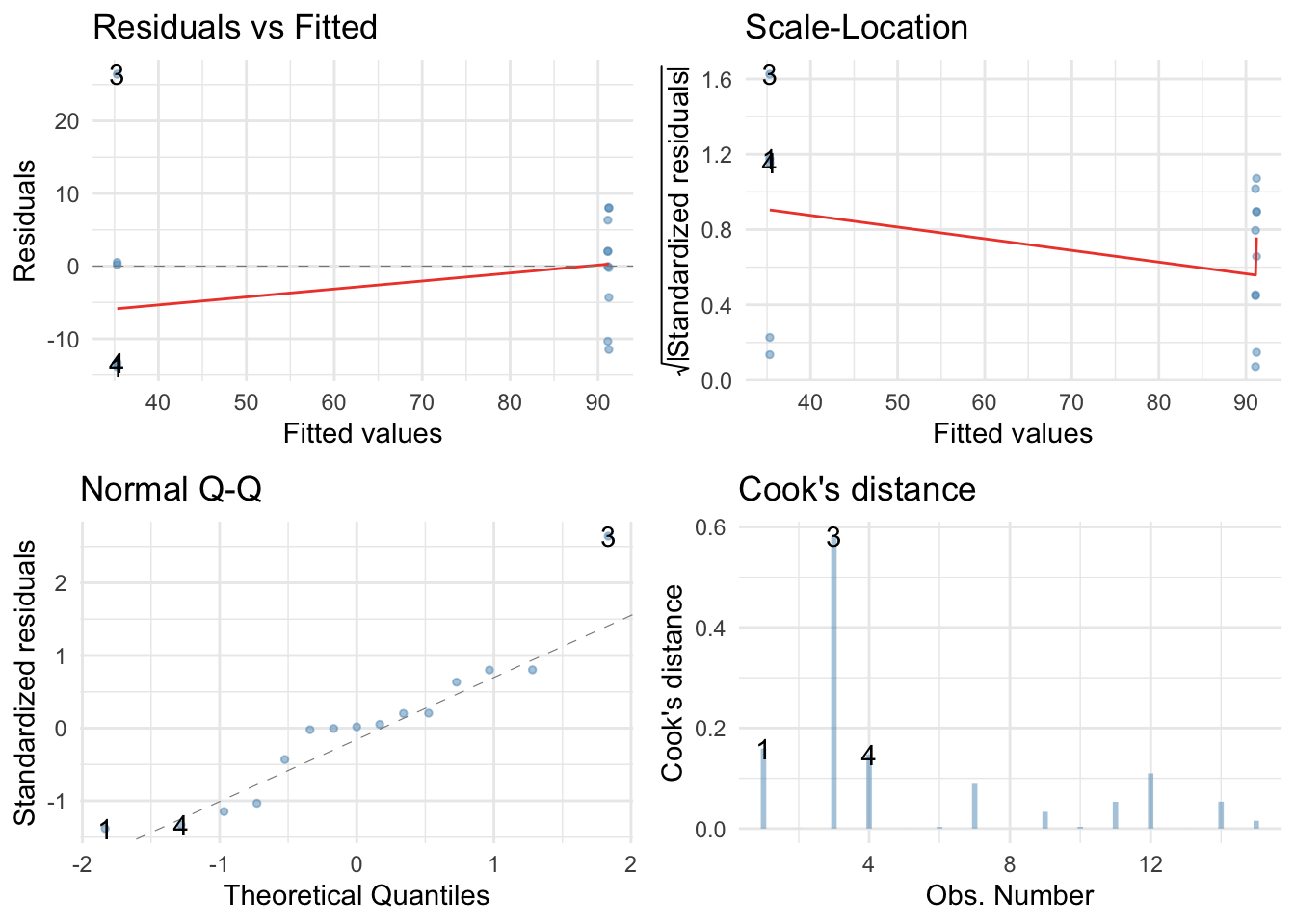
There are no large Cook’s distances, but the Q-Q plot suggests non-normal residuals and the resoidual vs fitted plot and the scale-location plot suggest heterogeneity of variance (the columns of dots are different lengths and the red line is not flat). Let’s fit a robust model.
oneway.test(displace ~ phallus, data = phallus_tib)
##
## 	One-way analysis of means (not assuming equal variances)
##
## data:  displace and phallus
## F = 24.488, num df = 2.0000, denom df = 7.3086, p-value = 0.0005758
The Welch F is highly significant still. Now the parameters:
parameters::model_parameters(phallus_lm, robust = TRUE, vcov.type = "HC4", digits = 3)
## Parameter                 | Coefficient |    SE |          95% CI |      t | df |      p
## ----------------------------------------------------------------------------------------
## (Intercept)               |      72.549 | 3.229 | [ 65.51, 79.58] | 22.470 | 12 | < .001
## phallusridge_vs_none      |      55.851 | 8.571 | [ 37.18, 74.53] |  6.516 | 12 | < .001
## phallusminimal_vs_coronal |       0.114 | 5.209 | [-11.24, 11.46] |  0.022 | 12 | 0.983
The first contrast is still highly significant and the second contrast highly non-significant. As such, our conclusions are unchanged when fitting a model that is robust to heteroscedasticity.
Eggs-traordinary
Load the data
To load the data from the CSV file (assuming you have set up a project folder as suggested in the book) and set the factors and the order of their levels:
eggs_tib <- readr::read_csv("../data/cetinkaya_2006.csv") %>%
  dplyr::mutate(
    groups = forcats::as_factor(groups) %>% forcats::fct_relevel(., "Fetishistics",    "NonFetishistics", "Control"),
    paired = forcats::as_factor(paired) %>% forcats::fct_relevel(., "Paired")
  )
Alternative, load the data directly from the discovr package:
eggs_tib <- discovr::cetinkaya_2006
The analysis in the paper
The authors conducted a Kruskal-Wallis test (a test not covered in the book because of our focus on robust methods). For the percentage of eggs, they report (p. 429):
Kruskal–Wallis analysis of variance (ANOVA) confirmed that female quail partnered with the different types of male quail produced different percentages of fertilized eggs, $ \chi^{2} $(2, N = 59) =11.95, p < .05, $ \eta^{2} $ = 0.20. Subsequent pairwise comparisons with the Mann–Whitney U test (with the Bonferroni correction) indicated that fetishistic male quail yielded higher rates of fertilization than both the nonfetishistic male quail (U = 56.00, N~1~ = 17, N~2~ = 15, effect size = 8.98, p < .05) and the control male quail (U= 100.00, N~1~ = 17, N~2~ = 27, effect size = 12.42, p < .05). However, the nonfetishistic group was not significantly different from the control group (U = 176.50, N~1~ = 15, N~2~ = 27, effect size = 2.69, p > .05).
For the latency data they reported as follows:
A Kruskal–Wallis analysis indicated significant group differences,$ \ \chi^{2} $(2, N = 59) = 32.24, p < .05, $ \eta^{2} $ = 0.56. Pairwise comparisons with the Mann–Whitney U test (with the Bonferroni correction) showed that the nonfetishistic males had significantly shorter copulatory latencies than both the fetishistic male quail (U = 0.00, N~1~ = 17, N~2~ = 15, effect size = 16.00, p < .05) and the control male quail (U = 12.00, N~1~ = 15, N~2~ = 27, effect size = 19.76, p < .05). However, the fetishistic group was not significantly different from the control group (U = 161.00, N~1~ = 17, N~2~ = 27, effect size = 6.57, p > .05). (p. 430)
These results support the authors' theory that fetishist behaviour may have evolved because it offers some adaptive function (such as preparing for the real thing).
Percentage of eggs
Let’s first plot some boxplots:
ggplot2::ggplot(eggs_tib, aes(groups, egg_percent)) +
  geom_boxplot(colour = "#5c97bf", fill = "#5c97bf", alpha = 0.4) +
  coord_cartesian(ylim = c(0, 100)) +
  scale_y_continuous(breaks = seq(0, 100, 10)) +
  labs(x = "Fetish group", y = "Percentage of eggs fertilised") +
  theme_minimal()
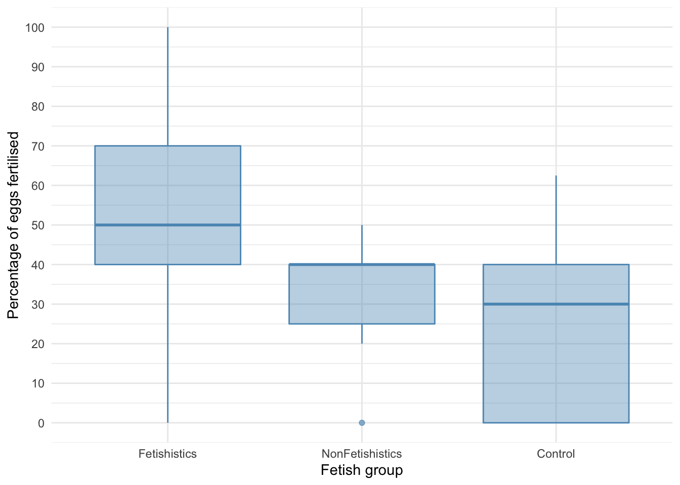
There is an outlier and skew in the non-fetishistic group and skew in the control group also. The authors were wise to fit a nonparametric test. We’ll use a 20% trimmed mean test with post hoc tests.
WRS2::t1way(egg_percent ~ groups, data = eggs_tib, nboot = 1000)
## Call:
## WRS2::t1way(formula = egg_percent ~ groups, data = eggs_tib,
##     nboot = 1000)
##
## Test statistic: F = 5.0223
## Degrees of freedom 1: 2
## Degrees of freedom 2: 22.2
## p-value: 0.01587
##
## Explanatory measure of effect size: 0.62
## Bootstrap CI: [0.22; 1.21]
The summary table tells us that there was a significant effect, F(2, 22.2) = 5.02, p = 0.016. Although we’ve applied a robust test rather than a nonparametric one the results of the study are confirmed. Let’s look at the post hoc tests:
WRS2::lincon(egg_percent ~ groups, data = eggs_tib)
## Call:
## WRS2::lincon(formula = egg_percent ~ groups, data = eggs_tib)
##
##                                    psihat  ci.lower ci.upper p.value
## Fetishistics vs. NonFetishistics 15.88745  -0.99058 32.76547 0.04785
## Fetishistics vs. Control         24.33516   3.76426 44.90606 0.01722
## NonFetishistics vs. Control       8.44771 -10.62899 27.52441 0.26796
There was no significant difference between the control group and the non-fetishistic group, $ \hat{\psi} = 8.45 [-10.63, 27.52]\text{, } p = 0.268 $, but significant differences were found between the control group and the fetishistic group, $ \hat{\psi} = 24.34 [3.76, 44.91]\text{, } p = 0.017 $, and between the fetishistic group and the non-fetishistic group, $ \hat{\psi} = 15.89 [-0.99, 32.77]\text{, } p = 0.0479 $. We know by looking at the boxplot (the medians in particular) that the fetishistic males yielded significantly higher rates of fertilization than both the non-fetishistic male quail and the control male quail. These results confirm the findings reported from the nonparametric tests in the paper.
Latency to copulate
Let’s first plot some boxplots:
ggplot2::ggplot(eggs_tib, aes(groups, latency)) +
  geom_boxplot(colour = "#5c97bf", fill = "#5c97bf", alpha = 0.4) +
  coord_cartesian(ylim = c(0, 60)) +
  scale_y_continuous(breaks = seq(0, 60, 10)) +
  labs(x = "Fetish group", y = "Latency to copulate (seconds)") +
  theme_minimal()
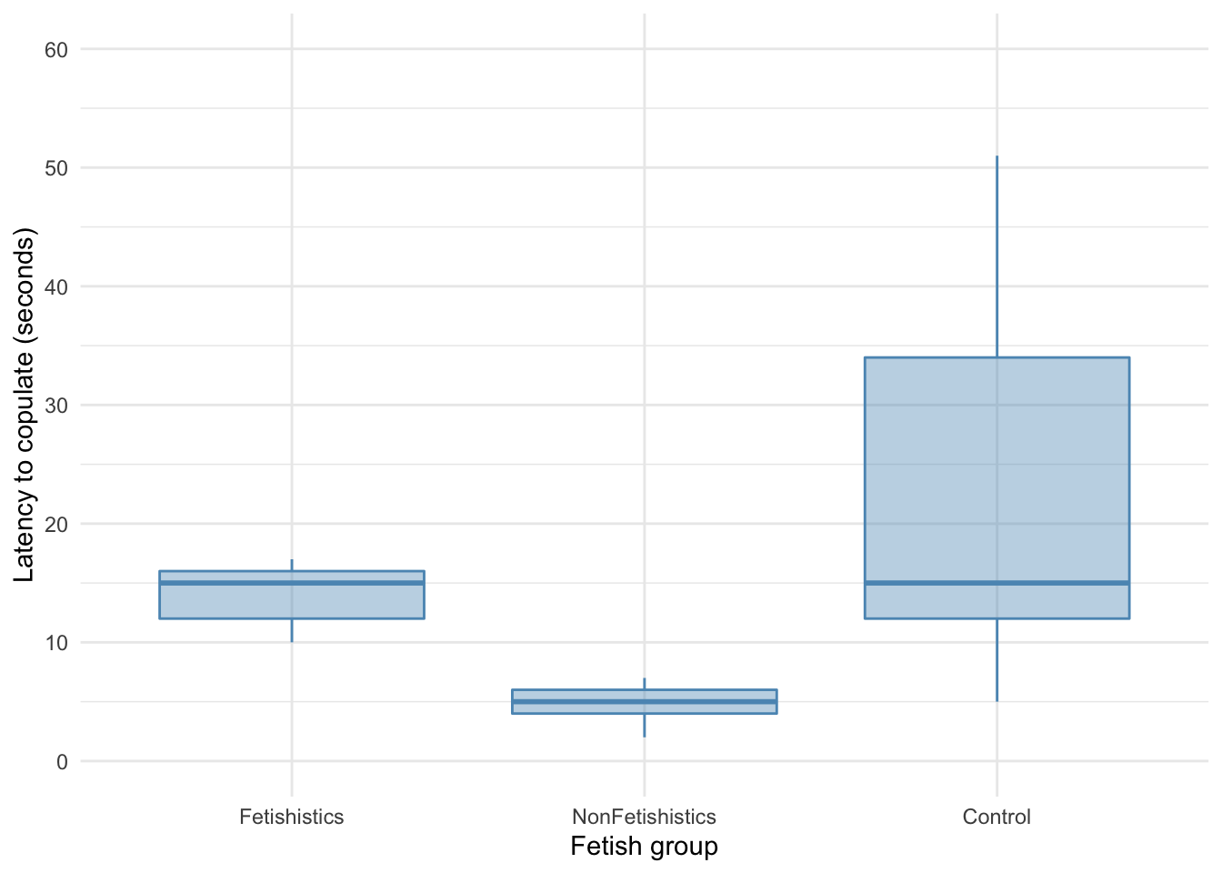
These groups have very different variances, which means the residuals will likely have too. As with the percentage of eggs, we’ll use a 20% trimmed mean test with post hoc tests.
WRS2::t1way(latency ~ groups, data = eggs_tib, nboot = 1000)
## Call:
## WRS2::t1way(formula = latency ~ groups, data = eggs_tib, nboot = 1000)
##
## Test statistic: F = 68.1179
## Degrees of freedom 1: 2
## Degrees of freedom 2: 21.28
## p-value: 0
##
## Explanatory measure of effect size: 1.11
## Bootstrap CI: [0.78; 1.65]
The summary table tells us that there was a significant effect, F(2, 21.28) = 68.12, p < 0.001. Although we’ve applied a robust test rather than a nonparametric one the results of the study are confirmed. Let’s look at the post hoc tests:
WRS2::lincon(latency ~ groups, data = eggs_tib)
Call: WRS2::lincon(formula = latency ~ groups, data = eggs_tib)
psihat ci.lower ci.upper p.value
Fetishistics vs. NonFetishistics 9.00000 6.87866 11.12134 0.00000 Fetishistics vs. Control -6.64706 -16.18974 2.89562 0.08419 NonFetishistics vs. Control -15.64706 -25.11973 -6.17439 0.00091 There was no significant difference between the control group and the fetishistic group, $ \hat{\psi} = -6.65 [-16.19, 2.90]\text{, } p = 0.084 $, but significant differences were found between the control group and the non-fetishistic group, $ \hat{\psi} = -15.65 [-25.12, -6.17]\text{, } p < 0.001 $, and between the fetishistic group and the non-fetishistic group, $ \hat{\psi} = 9.00 [6.88, 11.12]\text{, } p < 0.001 $. We know by looking at the boxplot (the medians in particular) that the non-fetishistic males yielded significantly lower rates of fertilization than the fetishistic male quail and the control male quail. Again, these results confirm the findings reported from the nonparametric tests in the paper.