Labcoat Leni solutions Chapter 9

This document contains abridged sections from Discovering Statistics Using R and RStudio by Andy Field so there are some copyright considerations. You can use this material for teaching and non-profit activities but please do not meddle with it or claim it as your own work. See the full license terms at the bottom of the page.
Bladder control
Load the file
tuk_tib <- readr::read_csv("../data/tuk_2011.csv") %>%
  dplyr::mutate(
    urgency = forcats::as_factor(urgency)
  )
Alternative, load the data directly from the discovr package:
tuk_tib <- discovr::tuk_2011
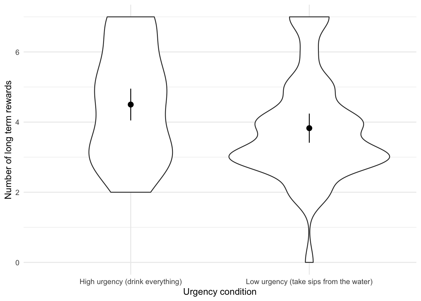
Plot a graph
ggplot2::ggplot(tuk_tib, aes(urgency, ll_sum)) +
  geom_violin() +
  stat_summary(fun.data = "mean_cl_normal") +
  labs(x = "Urgency condition", y = "Number of long term rewards") +
  theme_minimal()
Fit the model
We will conduct an independent samples t-test on these data because there were different participants in each of the two groups (independent design).
tuk_mod <- t.test(ll_sum ~ urgency, data = tuk_tib)
tuk_mod
##
## 	Welch Two Sample t-test
##
## data:  ll_sum by urgency
## t = 2.2001, df = 98.89, p-value = 0.03013
## alternative hypothesis: true difference in means is not equal to 0
## 95 percent confidence interval:
##  0.06603939 1.28011446
## sample estimates:
##        mean in group High urgency (drink everything)
##                                             4.500000
## mean in group Low urgency (take sips from the water)
##                                             3.826923
Looking at the means in the Group Statistics table below, we can see that on average more participants in the High Urgency group (M = 4.5) chose the large financial reward for which they would wait longer than participants in the low urgency group (M = 3.8). This difference was significant, p = .03.
To calculate the effect size d:
effectsize::cohens_d(ll_sum ~ urgency, data = tuk_tib)
## Cohen's d |       95% CI
## ------------------------
##      0.44 | [0.04, 0.83]
We could report this analysis as:
- On average, participants who had full bladders (M = 4.5, SD = 1.59) were more likely to choose the large financial reward for which they would wait longer than participants who had relatively empty bladders (M = 3.8, SD = 1.49), t(98.89) = 2.2, p = 0.03, d = 0.44, 0.95, 0.04, 0.83.
The beautiful people
Load the file
gelman_tib <- readr::read_csv("../data/gelman_2009.csv")
Alternative, load the data directly from the discovr package:
gelman_tib <- discovr::gelman_2009
Fit the model
We need to run a paired samples t-test on these data because the researchers recorded the number of daughters and sons for each participant (repeated-measures design). We need to make sure we sort the file by id so that the pairing is done correctly, and there are missing values so we need to set an action for dealing with those.
gelman_mod <- gelman_tib %>%
  dplyr::arrange(person) %>%
  t.test(number ~ child, data = ., paired = TRUE, na.action = "na.exclude")

gelman_mod
##
## 	Paired t-test
##
## data:  number by child
## t = -0.80702, df = 253, p-value = 0.4204
## alternative hypothesis: true difference in means is not equal to 0
## 95 percent confidence interval:
##  -0.20316864  0.08505841
## sample estimates:
## mean of the differences
##             -0.05905512
Looking at the output, we can see that there was a non-significant difference between the number of sons and daughters produced by the ‘beautiful’ celebrities.
To calculate the effect size d:
effectsize::cohens_d(number ~ child, data = gelman_tib)
## Cohen's d |        95% CI
## -------------------------
##     -0.07 | [-0.23, 0.10]
We could write up this analysis as follows:
- There was no significant difference between the number of daughters (M = 0.62, SE = 0.06) produced by the ‘beautiful’ celebrities and the number of sons (M = 0.68, SE = 0.06), t(253) = -0.807, p = 0.42, d = -0.07, 0.95, -0.23, 0.1.