Labcoat Leni solutions Chapter 8

This document contains abridged sections from Discovering Statistics Using R and RStudio by Andy Field so there are some copyright considerations. You can use this material for teaching and non-profit activities but please do not meddle with it or claim it as your own work. See the full license terms at the bottom of the page.
Load packages
Remember to load the tidyverse:
library(tidyverse)
I want to be loved (on Facebook)
Load the file
To load from the csv file use this code. Note that fct_relevel is used to ensure that factor levels match those in the original analysis.
ong_tib <- readr::read_csv("../data/chamorro_premuzic.csv") %>%
  dplyr::mutate(
    sex = forcats::as_factor(sex) %>% forcats::fct_relevel(., "Female"),
    grade = forcats::as_factor(grade) %>% forcats::fct_relevel(., "Sec 1", "Sec 2", "Sec 3")
  )
Alternative, load the data directly from the discovr package:
ong_tib <- discovr::ong_2011
Fit the models
The first linear model looks at whether narcissism predicts, above and beyond the other variables, the frequency of status updates. Fit this model:
ong_base_lm <- lm(status ~ sex + age + grade, data = ong_tib, na.action = na.exclude)
The second model adds extraversion:
ong_ext_lm <- update(ong_base_lm, .~. + extraversion)
The final mdoel adds narcissism:
ong_ncs_lm <- update(ong_ext_lm, .~. + narcissism)
Compare models
anova(ong_base_lm, ong_ext_lm, ong_ncs_lm) %>%
  broom::tidy() %>%
  knitr::kable(digits= 3)
| res.df | rss | df | sumsq | statistic | p.value |
|---|---|---|---|---|---|
| 246 | 1481.515 | NA | NA | NA | NA |
| 245 | 1458.360 | 1 | 23.155 | 4.017 | 0.046 |
| 244 | 1406.600 | 1 | 51.759 | 8.979 | 0.003 |
Adding extroversion and narcissim as predictors both significantly improve the fit of the model. (i.e. they are significant predictors.)
Model parameters:
ong_ncs_lm %>%
  parameters::model_parameters(standardize = "refit") %>%
  knitr::kable(digits = 3)
| Parameter | Coefficient | SE | CI_low | CI_high | t | df_error | p |
|---|---|---|---|---|---|---|---|
| (Intercept) | 0.381 | 0.211 | -0.035 | 0.797 | 1.805 | 244 | 0.072 |
| sexMale | -0.380 | 0.134 | -0.644 | -0.115 | -2.829 | 244 | 0.005 |
| age | -0.003 | 0.126 | -0.251 | 0.244 | -0.027 | 244 | 0.979 |
| gradeSec 2 | -0.169 | 0.211 | -0.584 | 0.245 | -0.804 | 244 | 0.422 |
| gradeSec 3 | -0.417 | 0.307 | -1.020 | 0.187 | -1.359 | 244 | 0.175 |
| extraversion | 0.026 | 0.070 | -0.113 | 0.165 | 0.367 | 244 | 0.714 |
| narcissism | 0.211 | 0.070 | 0.072 | 0.350 | 2.996 | 244 | 0.003 |
So basically, Ong et al.’s prediction was supported in that after adjusting for age, grade and gender, narcissism significantly predicted the frequency of Facebook status updates over and above extroversion. The positive standardized beta value (.21) indicates a positive relationship between frequency of Facebook updates and narcissism, in that more narcissistic adolescents updated their Facebook status more frequently than their less narcissistic peers did. Compare these results to the results reported in Ong et al. (2011). The Table 2 from their paper is reproduced at the end of this task below (look at the bottom section).
OK, now let’s fit more models to investigate whether narcissism predicts, above and beyond the other variables, the Facebook profile picture ratings. We use the same code as before but change the outcome from status to profile:
prof_base_lm <- lm(profile ~ sex + age + grade, data = ong_tib, na.action = na.exclude)
prof_ext_lm <- update(prof_base_lm, .~. + extraversion)
prof_ncs_lm <- update(prof_ext_lm, .~. + narcissism)
Compare models
anova(prof_base_lm, prof_ext_lm, prof_ncs_lm) %>%
  broom::tidy() %>%
  knitr::kable(digits = 3)
| res.df | rss | df | sumsq | statistic | p.value |
|---|---|---|---|---|---|
| 188 | 2405.233 | NA | NA | NA | NA |
| 187 | 2104.969 | 1 | 300.264 | 29.613 | 0 |
| 186 | 1885.958 | 1 | 219.011 | 21.600 | 0 |
Adding extraversion and narcissim as predictors both significantly improve the fit of the model. (i.e. they are significant predictors.)
Model parameters:
prof_ncs_lm %>%
  parameters::model_parameters(standardize = "refit") %>%
  knitr::kable(digits = 3)
| Parameter | Coefficient | SE | CI_low | CI_high | t | df_error | p |
|---|---|---|---|---|---|---|---|
| (Intercept) | 0.054 | 0.211 | -0.362 | 0.470 | 0.256 | 186 | 0.798 |
| sexMale | 0.162 | 0.146 | -0.127 | 0.450 | 1.104 | 186 | 0.271 |
| age | 0.099 | 0.123 | -0.144 | 0.341 | 0.801 | 186 | 0.424 |
| gradeSec 2 | -0.132 | 0.221 | -0.567 | 0.304 | -0.597 | 186 | 0.551 |
| gradeSec 3 | -0.155 | 0.302 | -0.751 | 0.441 | -0.515 | 186 | 0.607 |
| extraversion | 0.169 | 0.077 | 0.017 | 0.321 | 2.199 | 186 | 0.029 |
| narcissism | 0.368 | 0.079 | 0.212 | 0.524 | 4.648 | 186 | 0.000 |
These results show that after adjusting for age, grade and gender, narcissism significantly predicted the Facebook profile picture ratings over and above extroversion. The positive beta value (.37) indicates a positive relationship between profile picture ratings and narcissism, in that more narcissistic adolescents rated their Facebook profile pictures more positively than their less narcissistic peers did. Compare these results to the results reported in Table 2 of Ong et al. (2011) below.

Why do you like your lecturers?
Load the file
chamorro_tib <- readr::read_csv("../data/chamorro_premuzic.csv") %>%
  dplyr::mutate(
    sex = forcats::as_factor(sex)
  )
Alternative, load the data directly from the discovr package:
chamorro_tib <- discovr::chamorro_premuzic
Lecturer neuroticism
The first model we’ll fit predicts whether students want lecturers to be neurotic. In the first model put age and sex:
cp_neuro_lm <- lm(lec_neurotic ~ age + sex, data = chamorro_tib, na.action = na.exclude)
cp_neuro_lm %>%
  parameters::model_parameters(standardize = "refit") %>%
  knitr::kable(digits = 3)
| Parameter | Coefficient | SE | CI_low | CI_high | t | df_error | p |
|---|---|---|---|---|---|---|---|
| (Intercept) | -0.095 | 0.058 | -0.209 | 0.020 | -1.627 | 393 | 0.105 |
| age | 0.082 | 0.050 | -0.016 | 0.180 | 1.649 | 393 | 0.100 |
| sexMale | 0.344 | 0.111 | 0.126 | 0.563 | 3.100 | 393 | 0.002 |
In the next model block, put all of the student personality variables (five variables in all):
cp_neuro_full_lm <- lm(lec_neurotic ~ age + sex + stu_neurotic + stu_extro + stu_open + stu_agree + stu_consc, data = chamorro_tib, na.action = na.exclude)
cp_neuro_full_lm %>%
  broom::glance() %>%
  knitr::kable(digits = 3)
| r.squared | adj.r.squared | sigma | statistic | p.value | df | logLik | AIC | BIC | deviance | df.residual | nobs |
|---|---|---|---|---|---|---|---|---|---|---|---|
| 0.064 | 0.046 | 8.669 | 3.556 | 0.001 | 7 | -1330.799 | 2679.599 | 2714.893 | 27428.95 | 365 | 373 |
cp_neuro_full_lm %>%
  parameters::model_parameters(standardize = "refit") %>%
  knitr::kable(digits = 3)
| Parameter | Coefficient | SE | CI_low | CI_high | t | df_error | p |
|---|---|---|---|---|---|---|---|
| (Intercept) | -0.058 | 0.060 | -0.177 | 0.061 | -0.961 | 365 | 0.337 |
| age | 0.119 | 0.051 | 0.020 | 0.219 | 2.353 | 365 | 0.019 |
| sexMale | 0.214 | 0.122 | -0.026 | 0.455 | 1.754 | 365 | 0.080 |
| stu_neurotic | -0.059 | 0.058 | -0.173 | 0.055 | -1.022 | 365 | 0.307 |
| stu_extro | -0.078 | 0.055 | -0.186 | 0.030 | -1.428 | 365 | 0.154 |
| stu_open | -0.123 | 0.051 | -0.224 | -0.022 | -2.391 | 365 | 0.017 |
| stu_agree | 0.073 | 0.060 | -0.045 | 0.190 | 1.218 | 365 | 0.224 |
| stu_consc | -0.157 | 0.063 | -0.281 | -0.033 | -2.482 | 365 | 0.013 |
So basically, age, openness and conscientiousness were significant predictors of wanting a neurotic lecturer (note that for openness and conscientiousness the relationship is negative, i.e. the more a student scored on these characteristics, the less they wanted a neurotic lecturer).
Lecturer extroversion
The second variable we want to predict is lecturer extroversion. You can follow the steps of the first example but with the outcome variable of lec_extro:
cp_extro_lm <- lm(lec_extro ~ age + sex, data = chamorro_tib, na.action = na.exclude)
cp_extro_lm %>%
  parameters::model_parameters(standardize = "refit") %>%
  knitr::kable(digits = 3)
| Parameter | Coefficient | SE | CI_low | CI_high | t | df_error | p |
|---|---|---|---|---|---|---|---|
| (Intercept) | -0.036 | 0.069 | -0.172 | 0.101 | -0.511 | 279 | 0.610 |
| age | 0.013 | 0.060 | -0.105 | 0.131 | 0.216 | 279 | 0.829 |
| sexMale | 0.135 | 0.136 | -0.132 | 0.403 | 0.997 | 279 | 0.320 |
cp_extro_full_lm <- lm(lec_extro ~ age + sex + stu_neurotic + stu_extro + stu_open + stu_agree + stu_consc, data = chamorro_tib, na.action = na.exclude)
cp_extro_full_lm %>%
  broom::glance() %>%
  knitr::kable(digits = 3)
| r.squared | adj.r.squared | sigma | statistic | p.value | df | logLik | AIC | BIC | deviance | df.residual | nobs |
|---|---|---|---|---|---|---|---|---|---|---|---|
| 0.046 | 0.021 | 6.799 | 1.829 | 0.082 | 7 | -903.259 | 1824.518 | 1856.971 | 12204.22 | 264 | 272 |
cp_extro_full_lm %>%
  parameters::model_parameters(standardize = "refit") %>%
  knitr::kable(digits = 3)
| Parameter | Coefficient | SE | CI_low | CI_high | t | df_error | p |
|---|---|---|---|---|---|---|---|
| (Intercept) | -0.063 | 0.072 | -0.205 | 0.079 | -0.868 | 264 | 0.386 |
| age | 0.003 | 0.061 | -0.116 | 0.122 | 0.050 | 264 | 0.960 |
| sexMale | 0.230 | 0.147 | -0.060 | 0.520 | 1.562 | 264 | 0.119 |
| stu_neurotic | 0.022 | 0.072 | -0.120 | 0.163 | 0.305 | 264 | 0.761 |
| stu_extro | 0.155 | 0.066 | 0.024 | 0.286 | 2.338 | 264 | 0.020 |
| stu_open | 0.041 | 0.061 | -0.080 | 0.161 | 0.664 | 264 | 0.507 |
| stu_agree | 0.014 | 0.072 | -0.126 | 0.155 | 0.202 | 264 | 0.840 |
| stu_consc | 0.112 | 0.077 | -0.039 | 0.262 | 1.461 | 264 | 0.145 |
You should find that student extroversion was the only significant predictor of wanting an extrovert lecturer; the model overall did not explain a significant amount of the variance in wanting an extroverted lecturer.
Lecturer openness to experience
You can follow the steps of the first example but using lec_open as the outcome:
cp_open_lm <- lm(lec_open ~ age + sex, data = chamorro_tib, na.action = na.exclude)
cp_open_lm %>%
  parameters::model_parameters(standardize = "refit") %>%
  knitr::kable(digits = 3)
| Parameter | Coefficient | SE | CI_low | CI_high | t | df_error | p |
|---|---|---|---|---|---|---|---|
| (Intercept) | -0.002 | 0.059 | -0.118 | 0.114 | -0.040 | 396 | 0.968 |
| age | -0.015 | 0.050 | -0.114 | 0.084 | -0.299 | 396 | 0.765 |
| sexMale | 0.009 | 0.112 | -0.212 | 0.229 | 0.077 | 396 | 0.939 |
cp_open_full_lm <- lm(lec_open ~ age + sex + stu_neurotic + stu_extro + stu_open + stu_agree + stu_consc, data = chamorro_tib, na.action = na.exclude)
cp_open_full_lm %>%
  broom::glance() %>%
  knitr::kable(digits = 3)
| r.squared | adj.r.squared | sigma | statistic | p.value | df | logLik | AIC | BIC | deviance | df.residual | nobs |
|---|---|---|---|---|---|---|---|---|---|---|---|
| 0.064 | 0.046 | 7.921 | 3.604 | 0.001 | 7 | -1304.121 | 2626.242 | 2661.585 | 23025.6 | 367 | 375 |
cp_open_full_lm %>%
  parameters::model_parameters(standardize = "refit") %>%
  knitr::kable(digits = 3)
| Parameter | Coefficient | SE | CI_low | CI_high | t | df_error | p |
|---|---|---|---|---|---|---|---|
| (Intercept) | 0.007 | 0.060 | -0.111 | 0.126 | 0.122 | 367 | 0.903 |
| age | -0.019 | 0.051 | -0.118 | 0.081 | -0.370 | 367 | 0.712 |
| sexMale | -0.027 | 0.122 | -0.267 | 0.213 | -0.222 | 367 | 0.824 |
| stu_neurotic | 0.007 | 0.058 | -0.107 | 0.121 | 0.115 | 367 | 0.908 |
| stu_extro | 0.052 | 0.055 | -0.056 | 0.160 | 0.945 | 367 | 0.345 |
| stu_open | 0.217 | 0.051 | 0.116 | 0.318 | 4.238 | 367 | 0.000 |
| stu_agree | 0.133 | 0.059 | 0.016 | 0.250 | 2.232 | 367 | 0.026 |
| stu_consc | -0.051 | 0.063 | -0.175 | 0.073 | -0.813 | 367 | 0.417 |
You should find that student openness to experience was the most significant predictor of wanting a lecturer who is open to experience, but student agreeableness predicted this also.
Lecturer agreeableness
The fourth variable we want to predict is lecturer agreeableness. You can follow the steps of the first example but using lec_agree as the outcome:
cp_agree_lm <- lm(lec_agree ~ age + sex, data = chamorro_tib, na.action = na.exclude)
cp_agree_lm %>%
  parameters::model_parameters(standardize = "refit") %>%
  knitr::kable(digits = 3)
| Parameter | Coefficient | SE | CI_low | CI_high | t | df_error | p |
|---|---|---|---|---|---|---|---|
| (Intercept) | 0.017 | 0.058 | -0.097 | 0.132 | 0.294 | 393 | 0.769 |
| age | -0.169 | 0.050 | -0.267 | -0.071 | -3.399 | 393 | 0.001 |
| sexMale | -0.063 | 0.111 | -0.282 | 0.156 | -0.563 | 393 | 0.574 |
cp_agree_full_lm <- lm(lec_agree ~ age + sex + stu_neurotic + stu_extro + stu_open + stu_agree + stu_consc, data = chamorro_tib, na.action = na.exclude)
cp_agree_full_lm %>%
  broom::glance() %>%
  knitr::kable(digits = 3)
| r.squared | adj.r.squared | sigma | statistic | p.value | df | logLik | AIC | BIC | deviance | df.residual | nobs |
|---|---|---|---|---|---|---|---|---|---|---|---|
| 0.103 | 0.085 | 9.18 | 5.946 | 0 | 7 | -1348.537 | 2715.073 | 2750.343 | 30675.33 | 364 | 372 |
cp_agree_full_lm %>%
  parameters::model_parameters(standardize = "refit") %>%
  knitr::kable(digits = 3)
| Parameter | Coefficient | SE | CI_low | CI_high | t | df_error | p |
|---|---|---|---|---|---|---|---|
| (Intercept) | -0.028 | 0.059 | -0.144 | 0.088 | -0.474 | 364 | 0.636 |
| age | -0.175 | 0.050 | -0.273 | -0.077 | -3.520 | 364 | 0.000 |
| sexMale | 0.104 | 0.120 | -0.132 | 0.341 | 0.869 | 364 | 0.386 |
| stu_neurotic | 0.156 | 0.057 | 0.044 | 0.268 | 2.742 | 364 | 0.006 |
| stu_extro | 0.043 | 0.054 | -0.063 | 0.149 | 0.805 | 364 | 0.421 |
| stu_open | -0.141 | 0.050 | -0.240 | -0.041 | -2.790 | 364 | 0.006 |
| stu_agree | 0.132 | 0.059 | 0.017 | 0.248 | 2.255 | 364 | 0.025 |
| stu_consc | 0.072 | 0.062 | -0.050 | 0.194 | 1.161 | 364 | 0.246 |
You should find that Age, student openness to experience and student neuroticism significantly predicted wanting a lecturer who is agreeable. Age and openness to experience had negative relationships (the older and more open to experienced you are, the less you want an agreeable lecturer), whereas as student neuroticism increases so does the desire for an agreeable lecturer (not surprisingly, because neurotics will lack confidence and probably feel more able to ask an agreeable lecturer questions).
Lecturer conscientiousness
The final variable we want to predict is lecturer conscientiousness. You can follow the steps of the first example but replacing the outcome variable with lec_consc.
cp_consc_lm <- lm(lec_consc ~ age + sex, data = chamorro_tib, na.action = na.exclude)
cp_consc_lm %>%
  parameters::model_parameters(standardize = "refit") %>%
  knitr::kable(digits = 3)
| Parameter | Coefficient | SE | CI_low | CI_high | t | df_error | p |
|---|---|---|---|---|---|---|---|
| (Intercept) | 0.095 | 0.058 | -0.020 | 0.209 | 1.628 | 393 | 0.104 |
| age | 0.072 | 0.050 | -0.026 | 0.170 | 1.452 | 393 | 0.147 |
| sexMale | -0.348 | 0.112 | -0.567 | -0.128 | -3.117 | 393 | 0.002 |
cp_consc_full_lm <- lm(lec_consc ~ age + sex + stu_neurotic + stu_extro + stu_open + stu_agree + stu_consc, data = chamorro_tib, na.action = na.exclude)
cp_consc_full_lm %>%
  broom::glance() %>%
  knitr::kable(digits = 3)
| r.squared | adj.r.squared | sigma | statistic | p.value | df | logLik | AIC | BIC | deviance | df.residual | nobs |
|---|---|---|---|---|---|---|---|---|---|---|---|
| 0.074 | 0.056 | 7.259 | 4.132 | 0 | 7 | -1261.193 | 2540.387 | 2575.657 | 19180.05 | 364 | 372 |
cp_consc_full_lm %>%
  parameters::model_parameters(standardize = "refit") %>%
  knitr::kable(digits = 3)
| Parameter | Coefficient | SE | CI_low | CI_high | t | df_error | p |
|---|---|---|---|---|---|---|---|
| (Intercept) | 0.056 | 0.060 | -0.062 | 0.174 | 0.933 | 364 | 0.351 |
| age | 0.046 | 0.051 | -0.054 | 0.145 | 0.901 | 364 | 0.368 |
| sexMale | -0.209 | 0.122 | -0.450 | 0.032 | -1.706 | 364 | 0.089 |
| stu_neurotic | 0.012 | 0.058 | -0.101 | 0.126 | 0.212 | 364 | 0.832 |
| stu_extro | -0.059 | 0.055 | -0.166 | 0.049 | -1.076 | 364 | 0.283 |
| stu_open | -0.009 | 0.051 | -0.110 | 0.092 | -0.179 | 364 | 0.858 |
| stu_agree | 0.144 | 0.059 | 0.028 | 0.261 | 2.436 | 364 | 0.015 |
| stu_consc | 0.127 | 0.063 | 0.003 | 0.251 | 2.018 | 364 | 0.044 |
Student agreeableness and conscientiousness both signfiicantly predict wanting a lecturer who is conscientious. Note also that gender predicted this in the first step, but its b became slightly non-significant (p = .07) when the student personality variables were forced in as well. However, gender is probably a variable that should be explored further within this context.
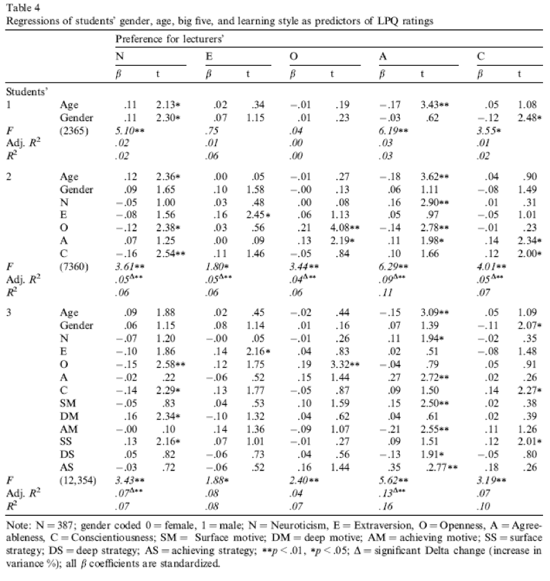
Compare all of your results to Table 4 in the actual article (shown below) - our five analyses are represented by the columns labelled N, E, O, A and C).