R code Chapter 18

Load packages
Remember to load the tidyverse:
library(tidyverse)
Load the data
Load the data from the discovr package:
raq_tib <- discovr::raq
If you want to read the file from the CSV and you have set up your project folder as I suggest in Chapter 1, then the code you would use is:
raq_tib <- here::here("data/raq.csv") %>%
  readr::read_csv()
Notice that the data file has a variable in it containing participants’ ids. We won’t want this variable in the analyses we do. Of course, we can use select() to remove it, but it will save a lot of repetitious code if we store a version of the data that only has the RAQ scores. We can do this with the following code:
raq_items_tib <- raq_tib %>%
  dplyr::select(-id)
We can create the correlations between variables by executing
raq_poly <- psych::polychoric(raq_items_tib)
raq_cor <- raq_poly$rho
We can view them using (to save space the code below isn’t executed)
round(raq_cor, 2)
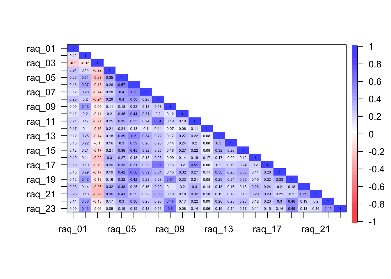
To get a plot of the correlations we can execute:
psych::cor.plot(raq_cor, upper = FALSE)
The Bartlett test
Conduct Bartlett’s test with either of these bits of code
psych::cortest.bartlett(raq_cor, n = 2571)
## $chisq
## [1] 17387.52
##
## $p.value
## [1] 0
##
## $df
## [1] 253
Determinant of the correlation matrix:
det(raq_cor)
## [1] 0.001127194
The KMO test
psych::KMO(raq_cor)
## Kaiser-Meyer-Olkin factor adequacy
## Call: psych::KMO(r = raq_cor)
## Overall MSA =  0.92
## MSA for each item =
## raq_01 raq_02 raq_03 raq_04 raq_05 raq_06 raq_07 raq_08 raq_09 raq_10 raq_11
##   0.95   0.94   0.93   0.93   0.95   0.91   0.96   0.86   0.84   0.95   0.89
## raq_12 raq_13 raq_14 raq_15 raq_16 raq_17 raq_18 raq_19 raq_20 raq_21 raq_22
##   0.90   0.95   0.96   0.96   0.92   0.90   0.95   0.93   0.93   0.93   0.94
## raq_23
##   0.84
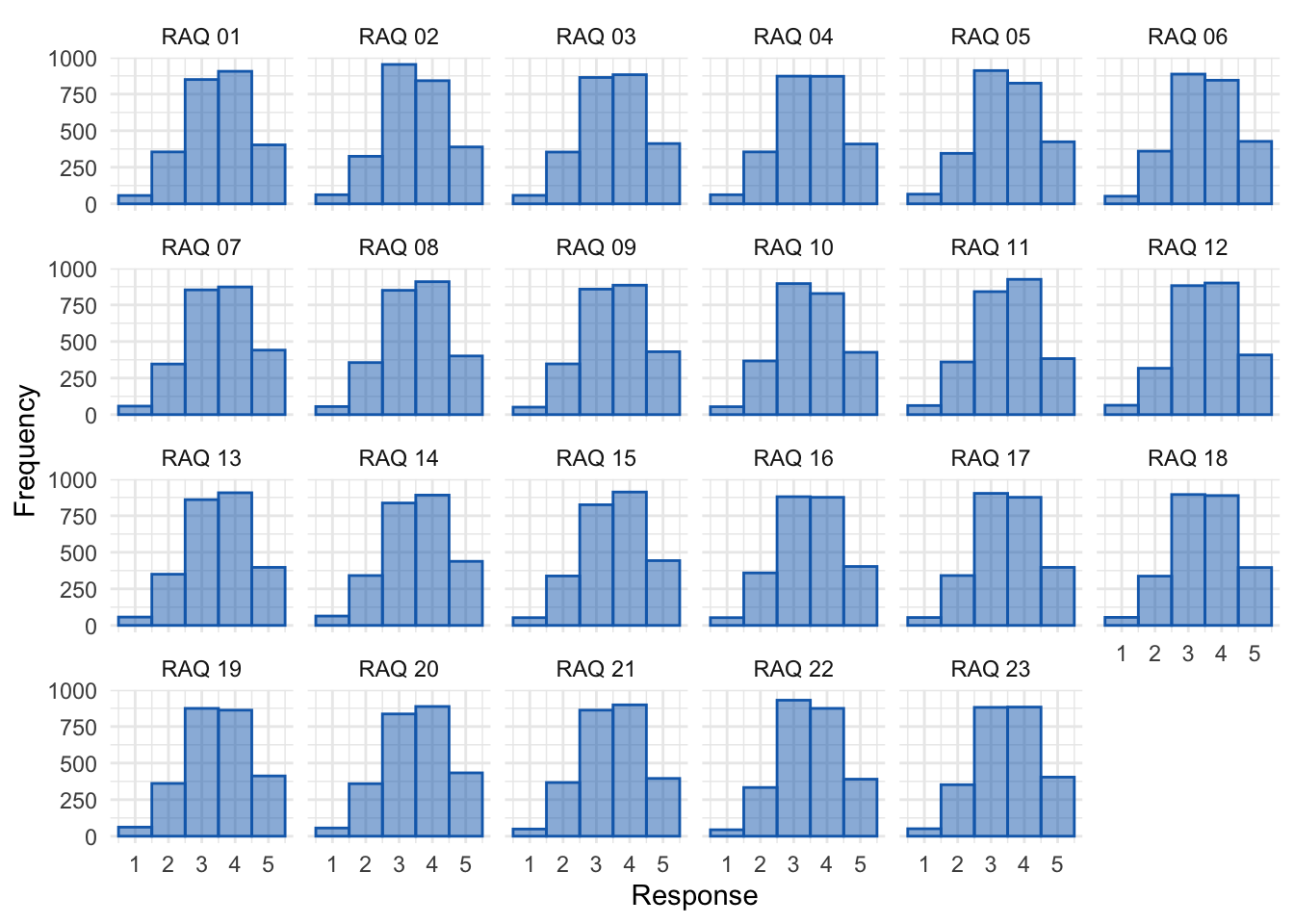
Self-test
raq_tidy_tib <- raq_items_tib %>%
  tidyr::pivot_longer(
    cols = raq_01:raq_23,
    names_to = "Item",
    values_to = "Response"
  ) %>%
  dplyr::mutate(
    Item = gsub("raq_", "RAQ ", Item)
  )

ggplot2::ggplot(raq_tidy_tib, aes(Response)) +
  geom_histogram(binwidth = 1, fill = "#136CB9", colour = "#136CB9", alpha = 0.5) +
  labs(y = "Frequency") +
  facet_wrap(~ Item, ncol = 6) +
  theme_minimal()
Parallel analysis
psych::fa.parallel(raq_cor, n.obs = 2571, fa = "fa")
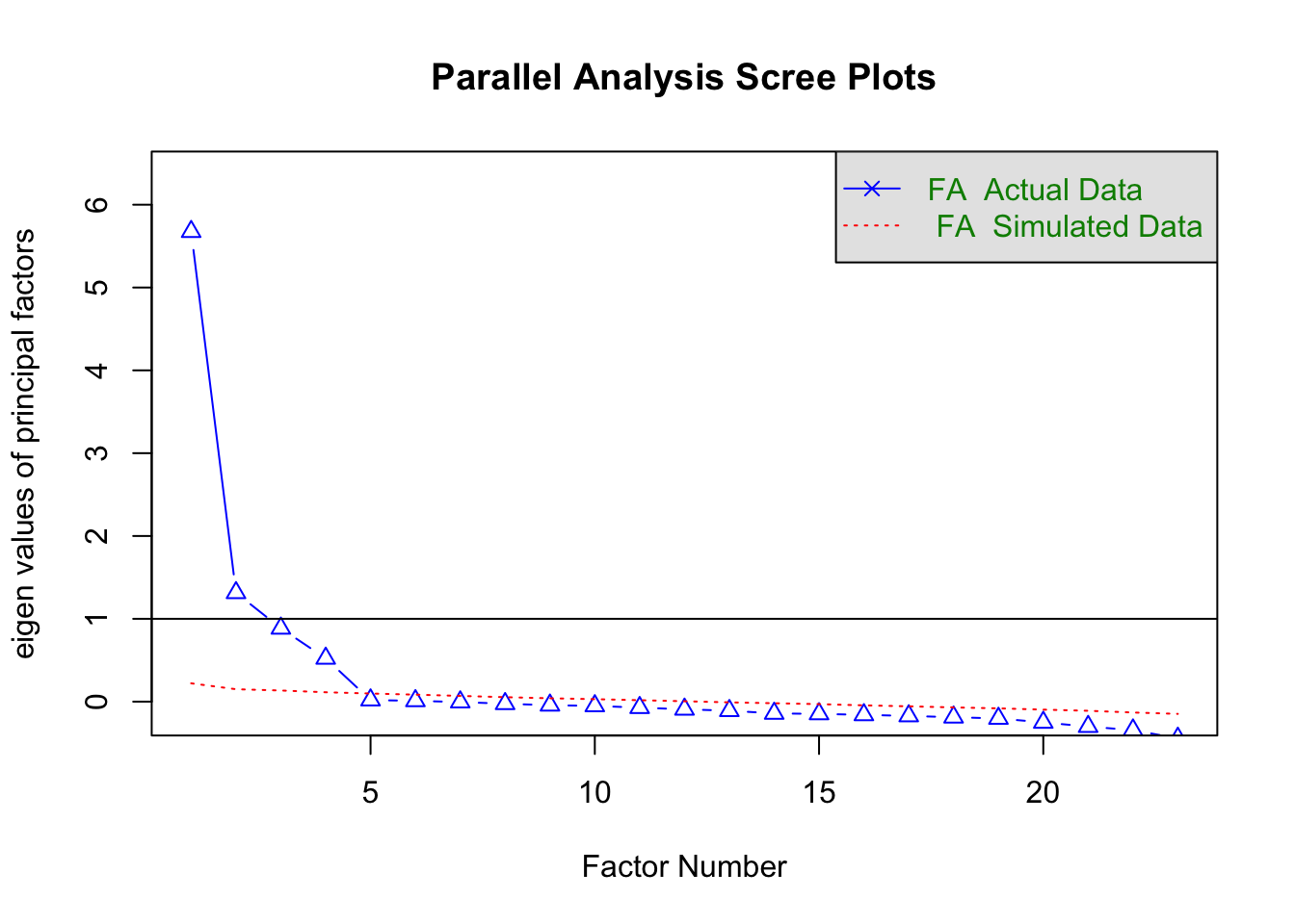
## Parallel analysis suggests that the number of factors = 4 and the number of components = NA
psych::fa.parallel(raq_cor, n.obs = 2571, fa = "pc")
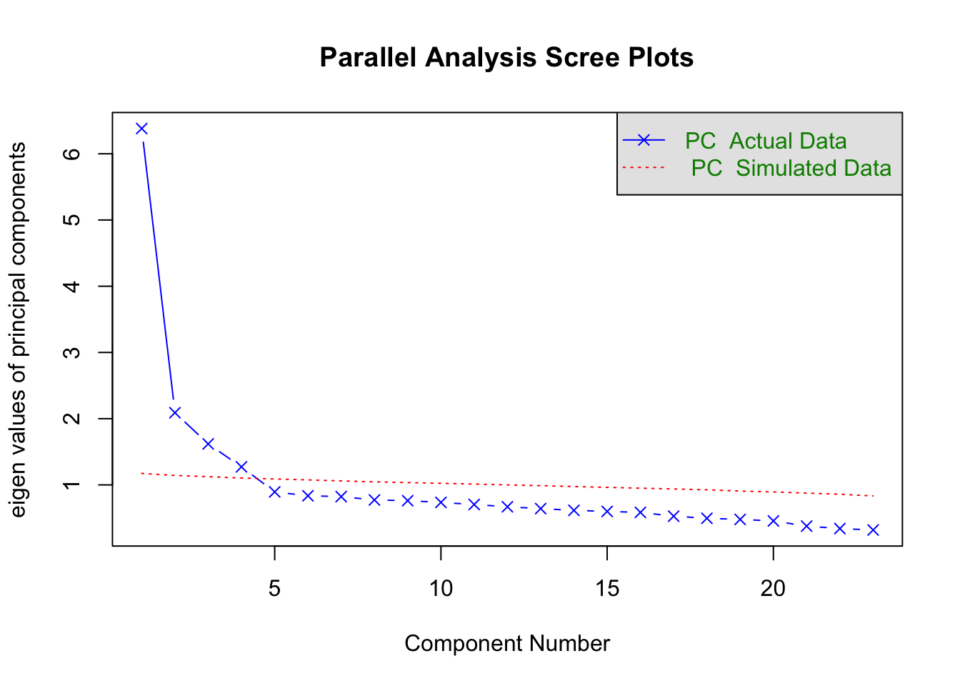
## Parallel analysis suggests that the number of factors = NA and the number of components = 4
Factor analysis
Create the factor analysis object.
From the raw data:
raq_fa <- psych::fa(raq_items_tib,
                    nfactors = 4,
                    scores = "tenBerge",
                    cor = "poly"
                    )
From the correlation matrix:
raq_fa <- psych::fa(raq_cor,
                    n.obs = 2571,
                    nfactors = 4,
                    scores = "tenBerge"
                    )
Inspect the residuals (not executed)
raq_cor
raq_fa$model
raq_fa$residual
To look only at the first 3 rows and the first 5 columns of these objects:
raq_cor[1:3, 1:5]
raq_fa$model[1:3, 1:5]
raq_fa$residual[1:3, 1:5]
raq_resids <- raq_fa$residual[upper.tri(raq_fa$residual)]

hist(raq_resids)
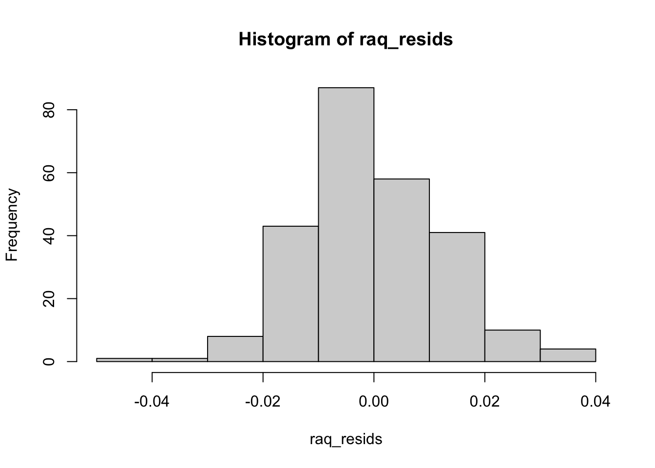
lge_resid_tot <- sum(abs(raq_resids) > 0.05)
lge_resid_tot
## [1] 0
lge_resid_pct <- lge_resid_tot/length(raq_resids)
lge_resid_pct
## [1] 0
rmsr <- raq_resids^2 %>% mean() %>% sqrt()
rmsr
## [1] 0.01255389
Piece of great
Wrap it into a function!
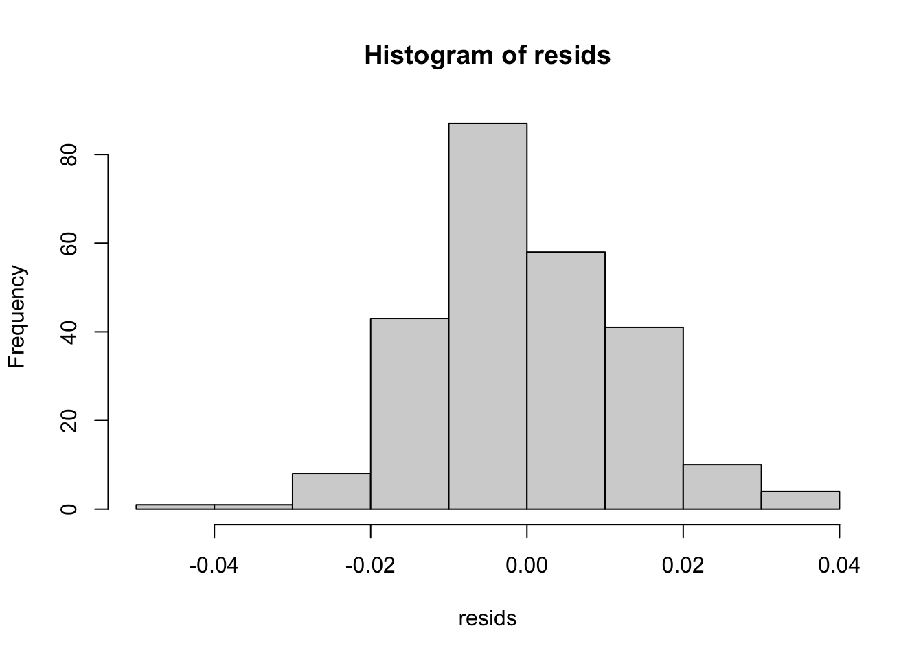
get_resids <- function(fa_object){
  resids <- fa_object$residual[upper.tri(fa_object$residual)]

  lge_resid_tot <- sum(abs(resids) > 0.05)
  lge_resid_pct <- 100*(lge_resid_tot/length(resids))
  rmsr <- sqrt(mean(resids^2))

  cat("Root means squared residual =", rmsr, "\n")
    cat("Number of absolute residuals > 0.05 =", lge_resid_tot, "\n")
    cat("Proportion of absolute residuals > 0.05 =", paste0(lge_resid_pct, "%"), "\n")
    hist(resids)
}

get_resids(raq_fa)
## Root means squared residual = 0.01255389
## Number of absolute residuals > 0.05 = 0
## Proportion of absolute residuals > 0.05 = 0%
Interpretation
Inspect the output:
raq_fa
## Factor Analysis using method =  minres
## Call: psych::fa(r = raq_cor, nfactors = 4, n.obs = 2571, scores = "tenBerge")
## Standardized loadings (pattern matrix) based upon correlation matrix
##          MR1   MR2   MR4   MR3   h2   u2 com
## raq_01 -0.03  0.01  0.39  0.06 0.17 0.83 1.1
## raq_02  0.25  0.48  0.02 -0.03 0.38 0.62 1.5
## raq_03  0.00  0.01 -0.43 -0.03 0.20 0.80 1.0
## raq_04  0.03 -0.02  0.56  0.00 0.33 0.67 1.0
## raq_05  0.45 -0.01  0.39  0.02 0.54 0.46 2.0
## raq_06  0.84  0.00 -0.01  0.03 0.73 0.27 1.0
## raq_07  0.56  0.04  0.00  0.04 0.35 0.65 1.0
## raq_08  0.00 -0.01 -0.01  0.88 0.75 0.25 1.0
## raq_09 -0.07  0.81  0.00  0.03 0.62 0.38 1.0
## raq_10  0.49 -0.05  0.09 -0.02 0.26 0.74 1.1
## raq_11 -0.01  0.01  0.03  0.72 0.55 0.45 1.0
## raq_12 -0.01  0.01  0.37 -0.07 0.11 0.89 1.1
## raq_13  0.57  0.03  0.04 -0.03 0.34 0.66 1.0
## raq_14  0.42  0.04  0.01  0.06 0.22 0.78 1.1
## raq_15  0.48  0.03  0.03  0.05 0.29 0.71 1.0
## raq_16 -0.05  0.02  0.51 -0.01 0.23 0.77 1.0
## raq_17  0.03  0.02  0.00  0.68 0.49 0.51 1.0
## raq_18  0.63  0.01 -0.02  0.07 0.43 0.57 1.0
## raq_19  0.26  0.56  0.00 -0.01 0.50 0.50 1.4
## raq_20  0.00  0.01  0.54  0.05 0.32 0.68 1.0
## raq_21 -0.02  0.05  0.59  0.06 0.40 0.60 1.0
## raq_22  0.19  0.52  0.03  0.05 0.41 0.59 1.3
## raq_23 -0.08  0.79  0.02 -0.01 0.59 0.41 1.0
##
##                        MR1  MR2  MR4  MR3
## SS loadings           3.04 2.24 2.03 1.91
## Proportion Var        0.13 0.10 0.09 0.08
## Cumulative Var        0.13 0.23 0.32 0.40
## Proportion Explained  0.33 0.24 0.22 0.21
## Cumulative Proportion 0.33 0.57 0.79 1.00
##
##  With factor correlations of
##      MR1  MR2  MR4  MR3
## MR1 1.00 0.38 0.50 0.48
## MR2 0.38 1.00 0.28 0.28
## MR4 0.50 0.28 1.00 0.57
## MR3 0.48 0.28 0.57 1.00
##
## Mean item complexity =  1.1
## Test of the hypothesis that 4 factors are sufficient.
##
## The degrees of freedom for the null model are  253  and the objective function was  6.79 with Chi Square of  17387.52
## The degrees of freedom for the model are 167  and the objective function was  0.1
##
## The root mean square of the residuals (RMSR) is  0.01
## The df corrected root mean square of the residuals is  0.02
##
## The harmonic number of observations is  2571 with the empirical chi square  205.03  with prob <  0.024
## The total number of observations was  2571  with Likelihood Chi Square =  267.21  with prob <  1.3e-06
##
## Tucker Lewis Index of factoring reliability =  0.991
## RMSEA index =  0.015  and the 90 % confidence intervals are  0.012 0.019
## BIC =  -1044.08
## Fit based upon off diagonal values = 1
## Measures of factor score adequacy
##                                                    MR1  MR2  MR4  MR3
## Correlation of (regression) scores with factors   0.93 0.91 0.88 0.92
## Multiple R square of scores with factors          0.87 0.83 0.77 0.85
## Minimum correlation of possible factor scores     0.73 0.66 0.54 0.70
Suppress some values and sort variables by their factor loading (method 1, not executed):
psych::print.psych(raq_fa, cut = 0.2, sort = TRUE)
Suppress some values and sort variables by their factor loading (method 2):
parameters::model_parameters(raq_fa, threshold = 0.2, sort = TRUE)
| Variable | MR1 | MR2 | MR4 | MR3 | Complexity | Uniqueness |
|---|---|---|---|---|---|---|
| raq_06 | 0.84 | 1.00 | 0.27 | |||
| raq_18 | 0.63 | 1.03 | 0.57 | |||
| raq_13 | 0.57 | 1.02 | 0.66 | |||
| raq_07 | 0.56 | 1.02 | 0.65 | |||
| raq_10 | 0.49 | 1.08 | 0.74 | |||
| raq_15 | 0.48 | 1.04 | 0.71 | |||
| raq_05 | 0.45 | 0.39 | 1.97 | 0.46 | ||
| raq_14 | 0.42 | 1.06 | 0.78 | |||
| raq_09 | 0.81 | 1.02 | 0.38 | |||
| raq_23 | 0.79 | 1.02 | 0.41 | |||
| raq_19 | 0.26 | 0.56 | 1.41 | 0.50 | ||
| raq_22 | 0.52 | 1.29 | 0.59 | |||
| raq_02 | 0.25 | 0.48 | 1.54 | 0.62 | ||
| raq_21 | 0.59 | 1.04 | 0.60 | |||
| raq_04 | 0.56 | 1.01 | 0.67 | |||
| raq_20 | 0.54 | 1.02 | 0.68 | |||
| raq_16 | 0.51 | 1.02 | 0.77 | |||
| raq_03 | -0.43 | 1.01 | 0.80 | |||
| raq_01 | 0.39 | 1.06 | 0.83 | |||
| raq_12 | 0.37 | 1.07 | 0.89 | |||
| raq_08 | 0.88 | 1.00 | 0.25 | |||
| raq_11 | 0.72 | 1.00 | 0.45 | |||
| raq_17 | 0.68 | 1.00 | 0.51 |
Factor scores
To view factor scores (not executed)
raq_fa$scores
Because we have 2571 cases, let’s look at only the first 10 rows using head():
raq_fa$scores %>% head(., 10)
## NULL
Reliability analysis
$ \omega_h $ and $ \omega_t $
raq_omg <- psych::omega(raq_items_tib,
                        nfactors = 4,
                        fm = "minres",
                        key = c(1, 1, -1, rep(1, 20)),
                        poly = TRUE
                        )
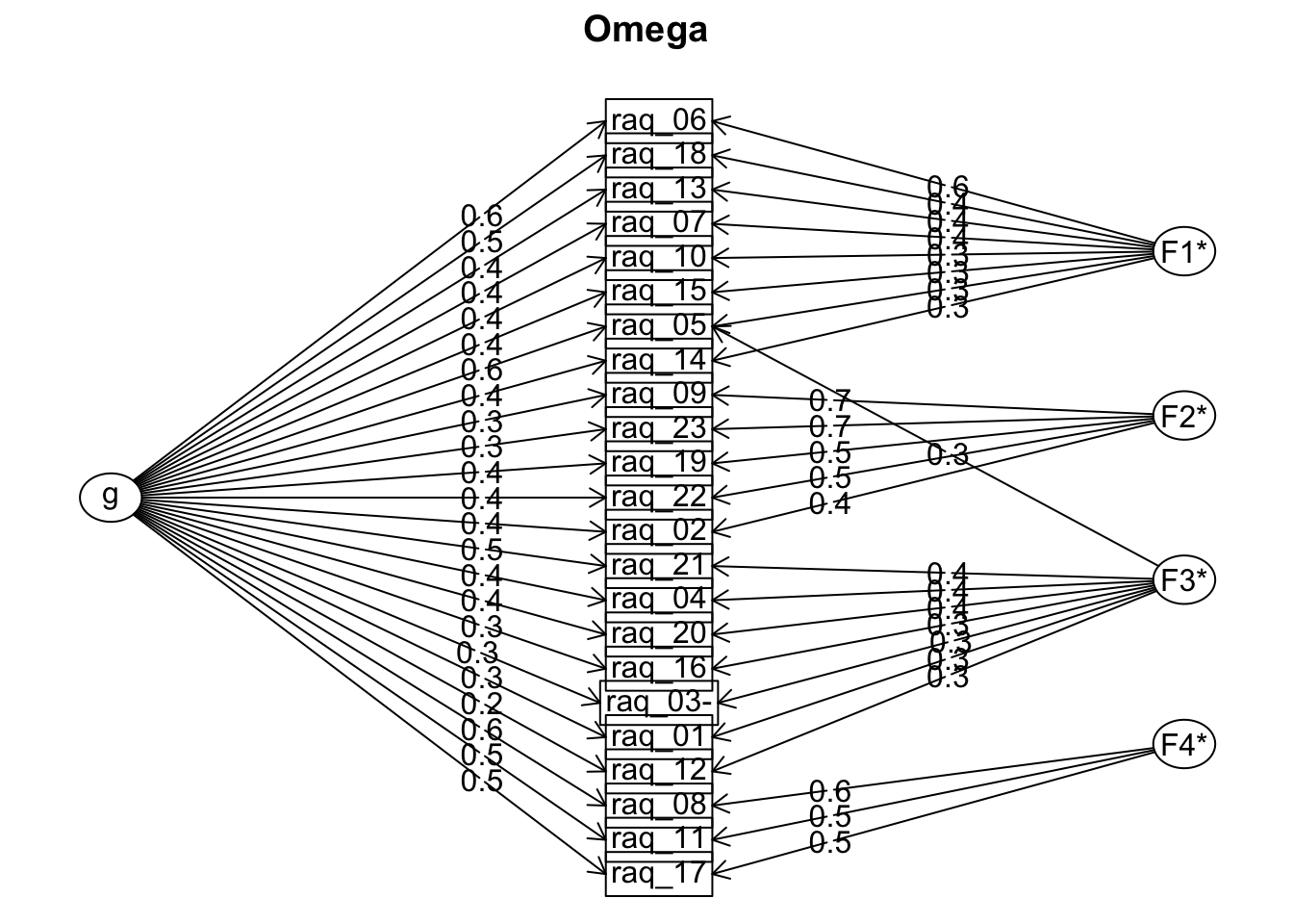
raq_omg
## Omega
## Call: omegah(m = m, nfactors = nfactors, fm = fm, key = key, flip = flip,
##     digits = digits, title = title, sl = sl, labels = labels,
##     plot = plot, n.obs = n.obs, rotate = rotate, Phi = Phi, option = option,
##     covar = covar)
## Alpha:                 0.88
## G.6:                   0.89
## Omega Hierarchical:    0.68
## Omega H asymptotic:    0.75
## Omega Total            0.9
##
## Schmid Leiman Factor loadings greater than  0.2
##            g   F1*   F2*   F3*   F4*   h2   u2   p2
## raq_01  0.32              0.26       0.17 0.83 0.57
## raq_02  0.37        0.43             0.38 0.62 0.37
## raq_03- 0.34              0.29       0.20 0.80 0.56
## raq_04  0.43              0.38       0.33 0.67 0.56
## raq_05  0.62  0.32        0.27       0.54 0.46 0.70
## raq_06  0.61  0.60                   0.73 0.27 0.51
## raq_07  0.44  0.39                   0.35 0.65 0.54
## raq_08  0.62                    0.61 0.75 0.25 0.51
## raq_09  0.32        0.73             0.62 0.38 0.17
## raq_10  0.37  0.35                   0.26 0.74 0.53
## raq_11  0.54                    0.50 0.55 0.45 0.54
## raq_12  0.22              0.25       0.11 0.89 0.44
## raq_13  0.42  0.40                   0.34 0.66 0.51
## raq_14  0.36  0.30                   0.22 0.78 0.59
## raq_15  0.41  0.34                   0.29 0.71 0.59
## raq_16  0.34              0.34       0.23 0.77 0.49
## raq_17  0.52                    0.47 0.49 0.51 0.55
## raq_18  0.48  0.44                   0.43 0.57 0.54
## raq_19  0.43        0.51             0.50 0.50 0.37
## raq_20  0.43              0.36       0.32 0.68 0.58
## raq_21  0.49              0.40       0.40 0.60 0.59
## raq_22  0.41        0.46             0.41 0.59 0.41
## raq_23  0.30        0.71             0.59 0.41 0.15
##
## With eigenvalues of:
##    g  F1*  F2*  F3*  F4*
## 4.40 1.39 1.71 0.85 0.86
##
## general/max  2.58   max/min =   2.01
## mean percent general =  0.49    with sd =  0.13 and cv of  0.26
## Explained Common Variance of the general factor =  0.48
##
## The degrees of freedom are 167  and the fit is  0.1
## The number of observations was  2571  with Chi Square =  267.21  with prob <  1.3e-06
## The root mean square of the residuals is  0.01
## The df corrected root mean square of the residuals is  0.02
## RMSEA index =  0.015  and the 10 % confidence intervals are  0.012 0.019
## BIC =  -1044.08
##
## Compare this with the adequacy of just a general factor and no group factors
## The degrees of freedom for just the general factor are 230  and the fit is  2.39
## The number of observations was  2571  with Chi Square =  6122.42  with prob <  0
## The root mean square of the residuals is  0.1
## The df corrected root mean square of the residuals is  0.11
##
## RMSEA index =  0.1  and the 10 % confidence intervals are  0.098 0.102
## BIC =  4316.45
##
## Measures of factor score adequacy
##                                                  g  F1*  F2*   F3*  F4*
## Correlation of scores with factors            0.84 0.76 0.87  0.67 0.74
## Multiple R square of scores with factors      0.71 0.57 0.75  0.44 0.55
## Minimum correlation of factor score estimates 0.42 0.14 0.51 -0.11 0.10
##
##  Total, General and Subset omega for each subset
##                                                  g  F1*  F2*  F3*  F4*
## Omega total for total scores and subscales    0.90 0.83 0.80 0.69 0.81
## Omega general for total scores and subscales  0.68 0.48 0.23 0.38 0.43
## Omega group for total scores and subscales    0.18 0.35 0.56 0.31 0.38
Cronbach’s $ \alpha $
There are lots of reasons not to use Cronbach’s $ \alpha $ (see the book for details). If you really must compute alpha then you need to compute it on the individual subscales. If the items are all scored in the same direction then we select the variables on a particular subscale and pipe them into psych::alpha(). For the fear of computers subscale
raq_tib %>%
  dplyr::select(raq_06, raq_07, raq_10, raq_13, raq_14, raq_15, raq_18) %>%
  psych::alpha()
For the Fear of peer/social evaluation subscale:
raq_tib %>%
  dplyr::select(raq_02, raq_09, raq_19, raq_22, raq_23) %>%
  psych::alpha()
##
## Reliability analysis
## Call: psych::alpha(x = .)
##
##   raw_alpha std.alpha G6(smc) average_r S/N    ase mean   sd median_r
##       0.78      0.78    0.75      0.42 3.6 0.0067  3.5 0.72     0.41
##
##  lower alpha upper     95% confidence boundaries
## 0.77 0.78 0.8
##
##  Reliability if an item is dropped:
##        raw_alpha std.alpha G6(smc) average_r S/N alpha se  var.r med.r
## raq_02      0.77      0.77    0.71      0.45 3.3   0.0075 0.0027  0.43
## raq_09      0.72      0.72    0.67      0.40 2.6   0.0089 0.0011  0.40
## raq_19      0.74      0.74    0.69      0.42 2.8   0.0084 0.0049  0.40
## raq_22      0.76      0.76    0.71      0.44 3.1   0.0078 0.0038  0.42
## raq_23      0.73      0.73    0.67      0.41 2.7   0.0086 0.0018  0.40
##
##  Item statistics
##           n raw.r std.r r.cor r.drop mean   sd
## raq_02 2571  0.68  0.69  0.55   0.49  3.5 0.97
## raq_09 2571  0.77  0.77  0.70   0.62  3.5 0.99
## raq_19 2571  0.74  0.74  0.64   0.57  3.5 1.00
## raq_22 2571  0.70  0.71  0.59   0.52  3.5 0.96
## raq_23 2571  0.76  0.76  0.68   0.60  3.5 0.98
##
## Non missing response frequency for each item
##           1    2    3    4    5 miss
## raq_02 0.02 0.13 0.37 0.33 0.15    0
## raq_09 0.02 0.13 0.33 0.34 0.17    0
## raq_19 0.02 0.14 0.34 0.34 0.16    0
## raq_22 0.02 0.13 0.36 0.34 0.15    0
## raq_23 0.02 0.14 0.34 0.34 0.16    0
For the Fear of mathematics subscale:
raq_tib %>%
  dplyr::select(raq_08, raq_11, raq_17) %>%
  psych::alpha()
##
## Reliability analysis
## Call: psych::alpha(x = .)
##
##   raw_alpha std.alpha G6(smc) average_r S/N    ase mean   sd median_r
##       0.77      0.77     0.7      0.53 3.4 0.0078  3.5 0.81     0.55
##
##  lower alpha upper     95% confidence boundaries
## 0.76 0.77 0.79
##
##  Reliability if an item is dropped:
##        raw_alpha std.alpha G6(smc) average_r S/N alpha se var.r med.r
## raq_08      0.63      0.63    0.47      0.47 1.7    0.014    NA  0.47
## raq_11      0.71      0.71    0.55      0.55 2.4    0.012    NA  0.55
## raq_17      0.74      0.74    0.58      0.58 2.8    0.010    NA  0.58
##
##  Item statistics
##           n raw.r std.r r.cor r.drop mean   sd
## raq_08 2571  0.86  0.86  0.75   0.66  3.5 0.98
## raq_11 2571  0.82  0.82  0.68   0.60  3.5 0.99
## raq_17 2571  0.81  0.81  0.65   0.57  3.5 0.97
##
## Non missing response frequency for each item
##           1    2    3    4    5 miss
## raq_08 0.02 0.14 0.33 0.35 0.16    0
## raq_11 0.02 0.14 0.33 0.36 0.15    0
## raq_17 0.02 0.13 0.35 0.34 0.15    0
Reverse scored-items
When a scale has reverse scored items, we need to tell the alpha() function which items are reversed by using the keys argument within the function. We supply this argument with a vector of 1s and -1s, which match the number of items on which we’re computing reliability. A 1 indicates a positively scored item and a -1 a negatively scored item. The Fear of statistics subscale has a reverse scored item: Standard deviations excite me (raq_03), so we need to indicate that this item is reverse scored.
For the fear of statistics subscale we could execute:
raq_tib %>%
  dplyr::select(raq_01, raq_03, raq_04, raq_05, raq_12, raq_16, raq_20, raq_21) %>%
  psych::alpha(keys = c(1, -1, 1, 1, 1, 1, 1, 1))
##
## Reliability analysis
## Call: psych::alpha(x = ., keys = c(1, -1, 1, 1, 1, 1, 1, 1))
##
##   raw_alpha std.alpha G6(smc) average_r S/N    ase mean   sd median_r
##       0.71      0.71    0.68      0.23 2.4 0.0087  3.4 0.57     0.22
##
##  lower alpha upper     95% confidence boundaries
## 0.69 0.71 0.72
##
##  Reliability if an item is dropped:
##         raw_alpha std.alpha G6(smc) average_r S/N alpha se  var.r med.r
## raq_01       0.69      0.69    0.67      0.24 2.2   0.0092 0.0050  0.24
## raq_03-      0.69      0.69    0.66      0.24 2.2   0.0094 0.0051  0.23
## raq_04       0.67      0.67    0.64      0.22 2.0   0.0100 0.0046  0.22
## raq_05       0.66      0.66    0.63      0.22 1.9   0.0102 0.0035  0.21
## raq_12       0.71      0.71    0.68      0.26 2.4   0.0088 0.0032  0.24
## raq_16       0.68      0.68    0.66      0.24 2.2   0.0095 0.0051  0.22
## raq_20       0.67      0.67    0.64      0.22 2.0   0.0099 0.0037  0.22
## raq_21       0.66      0.66    0.63      0.22 1.9   0.0103 0.0032  0.21
##
##  Item statistics
##            n raw.r std.r r.cor r.drop mean   sd
## raq_01  2571  0.52  0.52  0.39   0.33  3.5 0.99
## raq_03- 2571  0.54  0.54  0.42   0.36  2.5 0.99
## raq_04  2571  0.61  0.61  0.53   0.45  3.5 0.99
## raq_05  2571  0.64  0.64  0.58   0.48  3.5 1.00
## raq_12  2571  0.46  0.46  0.32   0.27  3.5 0.98
## raq_16  2571  0.55  0.55  0.44   0.37  3.5 0.98
## raq_20  2571  0.61  0.60  0.52   0.44  3.5 1.00
## raq_21  2571  0.64  0.65  0.58   0.49  3.5 0.98
##
## Non missing response frequency for each item
##           1    2    3    4    5 miss
## raq_01 0.02 0.14 0.33 0.35 0.16    0
## raq_03 0.02 0.14 0.34 0.34 0.16    0
## raq_04 0.02 0.14 0.34 0.34 0.16    0
## raq_05 0.03 0.13 0.35 0.32 0.16    0
## raq_12 0.02 0.12 0.34 0.35 0.16    0
## raq_16 0.02 0.14 0.34 0.34 0.16    0
## raq_20 0.02 0.14 0.33 0.35 0.17    0
## raq_21 0.02 0.14 0.34 0.35 0.15    0