R code Chapter 13
Load packages
Remember to load the tidyverse:
library(tidyverse)
Load the data
Load the data from the discover package:
goggles_tib <- discovr::goggles
If you want to read the file from the CSV and you have set up your project folder as I suggest in Chapter 1, then the code you would use is:
goggles_tib <- here::here("data/goggles.csv") %>%
  readr::read_csv() %>%
  dplyr::mutate(
    facetype = forcats::as_factor(facetype)
    alcohol = forcats::as_factor(alcohol)
  )
This code reads the file in and converts the variables facetype and alcohol to factors. It’s a good idea to check that the levels of facetype are in the order unattractive, attractive, and that the levels of alcohol are in the order placebo, low dose, high dose. Check the factor levels by executing:
levels(goggles_tib$facetype)
## [1] "Unattractive" "Attractive"
levels(goggles_tib$alcohol)
## [1] "Placebo" "Low dose" "High dose"
If they’re not in the correct order then:
goggles_tib <- goggles_tib %>%
    dplyr::mutate(
    facetype = forcats::fct_relevel(facetype, "Unattractive"),
    alcohol = forcats::fct_relevel(alcohol, "Placebo", "Low dose", "High dose")
  )
Self-test
Enter the data manually
goggles_tib <- tibble::tibble(
  id = c("vfnoxj", "hqfxap", "obicov", "oobiyc", "snafxn", "vihqnn", "ttrwbd", "anfyuf", "xwhodk", "nntqce", "vijnmk", "emutav", "cadtgo", "wpwfgy", "omvfpp", "xgyxnm", "troswv", "lygwvu", "aktinx", "xupshg", "ltmunk", "nywdas", "anbmps", "ailhsg", "ptalsm", "sbqkvb", "bdpjjq", "rwwpvm", "knkkfc", "eywqvv", "sawkng", "rsuarn", "iftwpu", "einkcx", "oawhad", "ouklsh", "siucar", "mjigqv", "enmsef", "rbrvsa", "ijklao", "oslboj", "yrbrqu", "viuvox", "efpdds", "ipwhor", "sbsxiw", "kkywwk"),
    facetype = gl(2, 24, labels = c("Attractive", "Unattractive")),
    alcohol = gl(3, 8, 48, labels = c("Placebo", "Low dose", "High dose")),
    attractiveness = c(6, 7, 6, 7, 6, 5, 8, 6, 7, 6, 8, 7, 6, 7, 6, 5, 5, 6, 7, 5, 7, 6, 5, 8, 2, 4, 3, 3, 4, 6, 5, 1, 3, 5, 7, 5, 4, 4, 5, 6, 5, 6, 8, 6, 7, 8, 7, 6)
    )
Plot the data
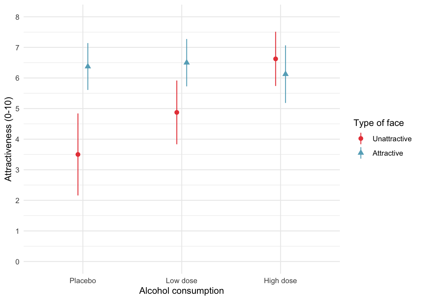
ggplot2::ggplot(goggles_tib, aes(x = alcohol, y = attractiveness, colour = facetype, shape = facetype)) +
  stat_summary(fun.data = "mean_cl_normal", geom = "pointrange", position = position_dodge(width = 0.2)) +
  coord_cartesian(ylim = c(0,8)) +
  scale_y_continuous(breaks = 0:8) +
  scale_colour_manual(values = c("#E84646", "#65ADC2")) +
  labs(x = "Alcohol consumption", y = "Attractiveness (0-10)", colour = "Type of face", shape = "Type of face") +
  theme_minimal()
Summary statistics
goggles_tib %>%
  dplyr::group_by(facetype, alcohol) %>%
  dplyr::summarize(
    mean = mean(attractiveness, na.rm = TRUE),
    `95% CI lower` = mean_cl_normal(attractiveness)$ymin,
    `95% CI upper` = mean_cl_normal(attractiveness)$ymax
  ) %>%
  knitr::kable(caption = "Summary statistics for the beer goggles data", digits = 2)
| facetype | alcohol | mean | 95% CI lower | 95% CI upper |
|---|---|---|---|---|
| Unattractive | Placebo | 3.50 | 2.16 | 4.84 |
| Unattractive | Low dose | 4.88 | 3.83 | 5.92 |
| Unattractive | High dose | 6.62 | 5.74 | 7.51 |
| Attractive | Placebo | 6.38 | 5.61 | 7.14 |
| Attractive | Low dose | 6.50 | 5.73 | 7.27 |
| Attractive | High dose | 6.12 | 5.18 | 7.07 |
Table 1: Summary statistics for the beer goggles data
Self-test
goggles_tib %>%
  dplyr::filter(alcohol != "Low dose") %>%
  lm(attractiveness ~ facetype*alcohol, data = .) %>%
  broom::tidy() %>%
  dplyr::mutate(
    across(where(is.numeric), ~round(., 3))
    )
## # A tibble: 4 x 5
##   term                                estimate std.error statistic p.value
##   <chr>                                  <dbl>     <dbl>     <dbl>   <dbl>
## 1 (Intercept)                             3.5      0.426      8.22       0
## 2 facetypeAttractive                      2.88     0.602      4.77       0
## 3 alcoholHigh dose                        3.12     0.602      5.19       0
## 4 facetypeAttractive:alcoholHigh dose    -3.38     0.852     -3.96       0
Fitting the model using afex::aov_4()
Raw analysis:
goggles_afx <- afex::aov_4(attractiveness ~ facetype*alcohol + (1|id), data = goggles_tib)
goggles_afx
## Anova Table (Type 3 tests)
##
## Response: attractiveness
##             Effect    df  MSE         F  ges p.value
## 1         facetype 1, 42 1.37 15.58 *** .271   <.001
## 2          alcohol 2, 42 1.37   6.04 ** .223    .005
## 3 facetype:alcohol 2, 42 1.37  8.51 *** .288   <.001
## ---
## Signif. codes:  0 '***' 0.001 '**' 0.01 '*' 0.05 '+' 0.1 ' ' 1
Correcting p-values:
goggles_afx <- afex::aov_4(attractiveness ~ facetype*alcohol + (1|id), data = goggles_tib, anova_table = list(p_adjust_method = "bonferroni"))
goggles_afx
## Anova Table (Type 3 tests, bonferroni-adjusted)
##
## Response: attractiveness
##             Effect    df  MSE         F  ges p.value
## 1         facetype 1, 42 1.37 15.58 *** .271   <.001
## 2          alcohol 2, 42 1.37    6.04 * .223    .015
## 3 facetype:alcohol 2, 42 1.37   8.51 ** .288    .002
## ---
## Signif. codes:  0 '***' 0.001 '**' 0.01 '*' 0.05 '+' 0.1 ' ' 1
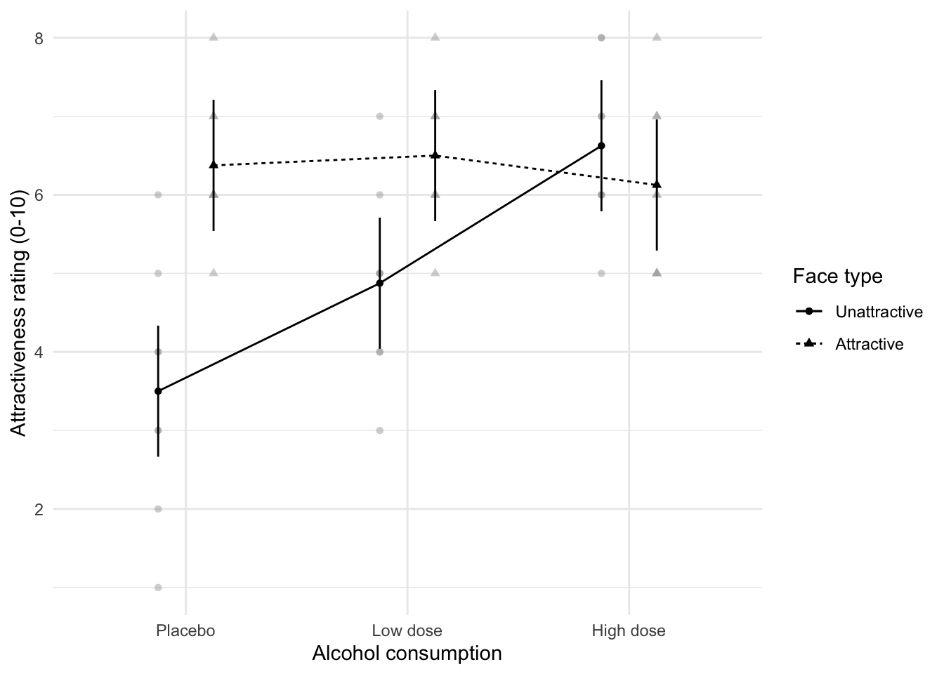
Plotting the data
afex::afex_plot(goggles_afx, "alcohol", "facetype", legend_title = "Face type") +
  labs(x = "Alcohol consumption", y = "Attractiveness rating (0-10)") +
  theme_minimal()
Fitting the model using lm()
Set contrasts for facetype:
unatt_vs_att <- c(-0.5, 0.5)
contrasts(goggles_tib$facetype) <- unatt_vs_att
Set contrasts for alcohol:
none_vs_alcohol <- c(-2/3, 1/3, 1/3)
low_vs_high <- c(0, -1/2, 1/2)
contrasts(goggles_tib$alcohol) <- cbind(none_vs_alcohol, low_vs_high)
Check the contrasts:
contrasts(goggles_tib$facetype)
##              [,1]
## Unattractive -0.5
## Attractive    0.5
contrasts(goggles_tib$alcohol)
##           none_vs_alcohol low_vs_high
## Placebo        -0.6666667         0.0
## Low dose        0.3333333        -0.5
## High dose       0.3333333         0.5
Fit the model and print Type III sums of squares:
goggles_lm <- lm(attractiveness ~ facetype*alcohol, data = goggles_tib)
car::Anova(goggles_lm, type = 3)
## Anova Table (Type III tests)
##
## Response: attractiveness
##                   Sum Sq Df   F value    Pr(>F)
## (Intercept)      1541.33  1 1125.8435 < 2.2e-16 ***
## facetype           21.33  1   15.5826 0.0002952 ***
## alcohol            16.54  2    6.0413 0.0049434 **
## facetype:alcohol   23.29  2    8.5065 0.0007913 ***
## Residuals          57.50 42
## ---
## Signif. codes:  0 '***' 0.001 '**' 0.01 '*' 0.05 '.' 0.1 ' ' 1
Interpreting effects
Self test
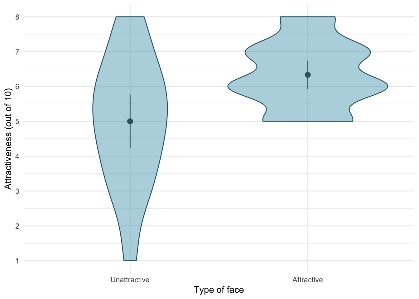
Plot the main effect of type of face
ggplot2::ggplot(goggles_tib, aes(x = facetype, y= attractiveness)) +
  geom_violin(colour = "#316675", fill = "#65ADC2", alpha = 0.5) +
  stat_summary(fun.data = "mean_cl_normal", colour = "#316675") +
  scale_y_continuous(breaks = 0:8) +
  labs(y = "Attractiveness (out of 10)", x = "Type of face") +
  theme_minimal()
Getting the estimated marginal means for the model created using afex::aov_4()
emmeans::emmeans(goggles_afx, "facetype")
##  facetype     emmean    SE df lower.CL upper.CL
##  Unattractive   5.00 0.239 42     4.52     5.48
##  Attractive     6.33 0.239 42     5.85     6.82
##
## Results are averaged over the levels of: alcohol
## Confidence level used: 0.95
Getting the estimated marginal means for the model created using lm()
emmeans::emmeans(goggles_lm, "facetype")
##  facetype     emmean    SE df lower.CL upper.CL
##  Unattractive   5.00 0.239 42     4.52     5.48
##  Attractive     6.33 0.239 42     5.85     6.82
##
## Results are averaged over the levels of: alcohol
## Confidence level used: 0.95
Self test
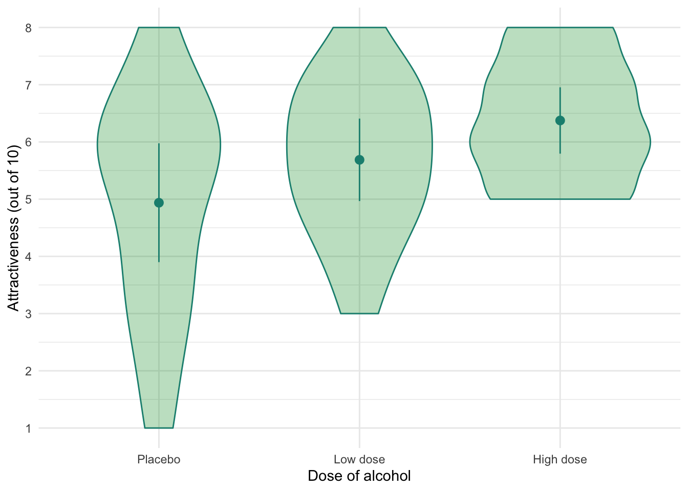
Plot the main effect of alcohol consumption
ggplot2::ggplot(goggles_tib, aes(x = alcohol, y= attractiveness)) +
  geom_violin(colour = "#168E7F", fill = "#109B37", alpha = 0.3) +
  stat_summary(fun.data = "mean_cl_normal", colour = "#168E7F") +
  scale_y_continuous(breaks = 0:8) +
  labs(y = "Attractiveness (out of 10)", x = "Dose of alcohol") +
  theme_minimal()
Get estimated marginal means from the afex::aov_4() model
emmeans::emmeans(goggles_afx, "alcohol")
##  alcohol   emmean    SE df lower.CL upper.CL
##  Placebo     4.94 0.293 42     4.35     5.53
##  Low dose    5.69 0.293 42     5.10     6.28
##  High dose   6.38 0.293 42     5.78     6.97
##
## Results are averaged over the levels of: facetype
## Confidence level used: 0.95
Get estimated marginal means from the `lm’ model
emmeans::emmeans(goggles_lm, "alcohol")
##  alcohol   emmean    SE df lower.CL upper.CL
##  Placebo     4.94 0.293 42     4.35     5.53
##  Low dose    5.69 0.293 42     5.10     6.28
##  High dose   6.38 0.293 42     5.78     6.97
##
## Results are averaged over the levels of: facetype
## Confidence level used: 0.95
Plot the interaction using afex
afex::afex_plot(goggles_afx, "alcohol", "facetype", legend_title = "Face type") +
  labs(x = "Alcohol consumption", y = "Attractiveness rating (0-10)") +
  theme_minimal()

Get estimated marginal means from the afex::aov_4() model
emmeans::emmeans(goggles_afx, c("alcohol", "facetype"))
##  alcohol   facetype     emmean    SE df lower.CL upper.CL
##  Placebo   Unattractive   3.50 0.414 42     2.67     4.33
##  Low dose  Unattractive   4.88 0.414 42     4.04     5.71
##  High dose Unattractive   6.62 0.414 42     5.79     7.46
##  Placebo   Attractive     6.38 0.414 42     5.54     7.21
##  Low dose  Attractive     6.50 0.414 42     5.67     7.33
##  High dose Attractive     6.12 0.414 42     5.29     6.96
##
## Confidence level used: 0.95
Get estimated marginal means from the lm() model
emmeans::emmeans(goggles_lm, c("alcohol", "facetype"))
##  alcohol   facetype     emmean    SE df lower.CL upper.CL
##  Placebo   Unattractive   3.50 0.414 42     2.67     4.33
##  Low dose  Unattractive   4.88 0.414 42     4.04     5.71
##  High dose Unattractive   6.62 0.414 42     5.79     7.46
##  Placebo   Attractive     6.38 0.414 42     5.54     7.21
##  Low dose  Attractive     6.50 0.414 42     5.67     7.33
##  High dose Attractive     6.12 0.414 42     5.29     6.96
##
## Confidence level used: 0.95
Contrasts
View the contrasts set for the model fitted with lm()
broom::tidy(goggles_lm, conf.int = TRUE) %>%
  dplyr::mutate(
    across(where(is.numeric), ~round(., 3))
  )
## # A tibble: 6 x 7
##   term                   estimate std.error statistic p.value conf.low conf.high
##   <chr>                     <dbl>     <dbl>     <dbl>   <dbl>    <dbl>     <dbl>
## 1 (Intercept)               5.67      0.169     33.6    0        5.33      6.01
## 2 facetype1                 1.33      0.338      3.95   0        0.652     2.02
## 3 alcoholnone_vs_alcohol    1.09      0.358      3.05   0.004    0.371     1.82
## 4 alcohollow_vs_high        0.687     0.414      1.66   0.104   -0.147     1.52
## 5 facetype1:alcoholnone…   -2.31      0.717     -3.23   0.002   -3.76     -0.867
## 6 facetype1:alcohollow_…   -2.12      0.827     -2.57   0.014   -3.80     -0.455
Simple effects
To look at the effect of facetype at each level of alcohol, we’d execute:
emmeans::joint_tests(goggles_afx, "alcohol")
## alcohol = Placebo:
##  model term df1 df2 F.ratio p.value
##  facetype     1  42  24.150 <.0001
##
## alcohol = Low dose:
##  model term df1 df2 F.ratio p.value
##  facetype     1  42   7.715 0.0081
##
## alcohol = High dose:
##  model term df1 df2 F.ratio p.value
##  facetype     1  42   0.730 0.3976
or for the model created with lm()
emmeans::joint_tests(goggles_lm, "alcohol")
To look at the effect of alcohol at each level of facetype, we’d execute:
emmeans::joint_tests(goggles_afx, "facetype")
## facetype = Unattractive:
##  model term df1 df2 F.ratio p.value
##  alcohol      2  42  14.335 <.0001
##
## facetype = Attractive:
##  model term df1 df2 F.ratio p.value
##  alcohol      2  42   0.213 0.8090
or for the model created with lm()
emmeans::joint_tests(goggles_lm, "facetype")
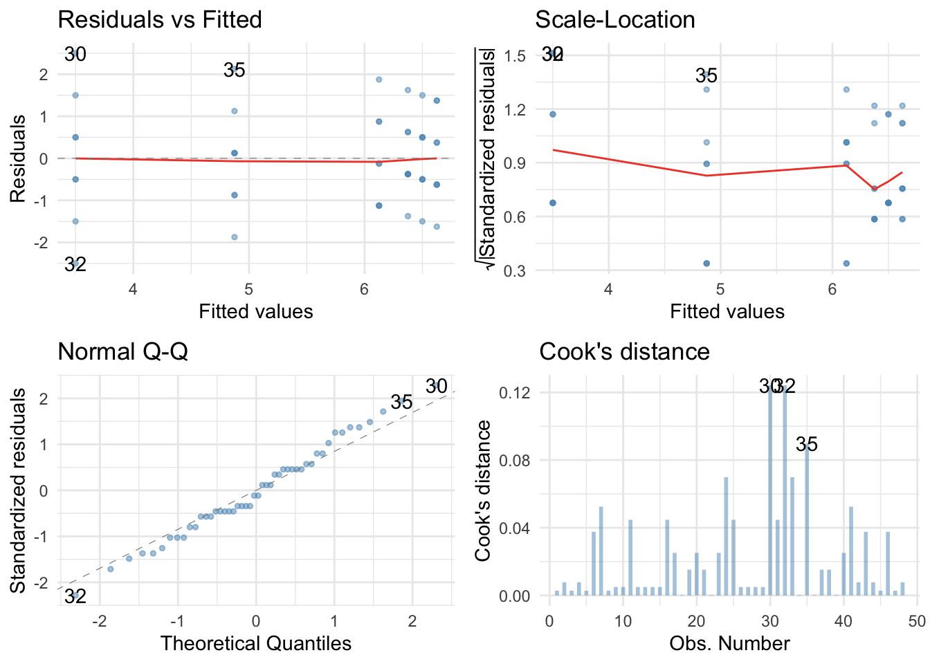
Self test: Diagnostic plots
Plot residuals from the goggles_lm model. Remember to execute library(ggfortify) before running this code.
ggplot2::autoplot(goggles_lm,
                  which = c(1, 3, 2, 4),
                  colour = "#5c97bf",
                  smooth.colour = "#ef4836",
                  alpha = 0.5,
                  size = 1) +
  theme_minimal()
Robust models
Self-test
Fit a model using lmRob()
goggles_rob <- robust::lmRob(attractiveness ~ facetype*alcohol, data = goggles_tib)
summary(goggles_rob)
##
## Call:
## robust::lmRob(formula = attractiveness ~ facetype * alcohol,
##     data = goggles_tib)
##
## Residuals:
##    Min     1Q Median     3Q    Max
## -2.500 -0.625 -0.125  0.625  2.500
##
## Coefficients:
##                                  Estimate Std. Error t value Pr(>|t|)
## (Intercept)                        5.6667     0.1954  29.000  < 2e-16 ***
## facetype1                          1.3333     0.3908   3.412  0.00144 **
## alcoholnone_vs_alcohol             1.0938     0.4215   2.595  0.01298 *
## alcohollow_vs_high                 0.6875     0.4704   1.461  0.15133
## facetype1:alcoholnone_vs_alcohol  -2.3125     0.8430  -2.743  0.00891 **
## facetype1:alcohollow_vs_high      -2.1250     0.9408  -2.259  0.02916 *
## ---
## Signif. codes:  0 '***' 0.001 '**' 0.01 '*' 0.05 '.' 0.1 ' ' 1
##
## Residual standard error: 1.339 on 42 degrees of freedom
## Multiple R-Squared: 0.439
##
## Test for Bias:
##             statistic p-value
## M-estimate    -0.5931       1
## LS-estimate   -6.9320       1
Robust standard errors
HC4 standard errors
parameters::model_parameters(goggles_lm, robust = TRUE, vcov.type = "HC4", digits = 3)
## Parameter                                | Coefficient |    SE |         95% CI |  t(42) |      p
## -------------------------------------------------------------------------------------------------
## (Intercept)                              |       5.667 | 0.181 | [ 5.30,  6.03] | 31.387 | < .001
## facetype [1]                             |       1.333 | 0.361 | [ 0.60,  2.06] |  3.693 | < .001
## alcohol [none_vs_alcohol]                |       1.094 | 0.406 | [ 0.27,  1.91] |  2.695 | 0.010
## alcohol [low_vs_high]                    |       0.687 | 0.414 | [-0.15,  1.52] |  1.660 | 0.104
## facetype [1] * alcohol [none_vs_alcohol] |      -2.313 | 0.812 | [-3.95, -0.67] | -2.849 | 0.007
## facetype [1] * alcohol [low_vs_high]     |      -2.125 | 0.828 | [-3.80, -0.45] | -2.565 | 0.014
Bootstrap standard errors
parameters::bootstrap_parameters(goggles_lm)
## # Fixed Effects
##
## Parameter                        | Coefficient |         95% CI |     p
## -----------------------------------------------------------------------
## (Intercept)                      |        5.68 | [ 5.36,  6.00] | 0.001
## facetype1                        |        1.33 | [ 0.62,  1.95] | 0.001
## alcoholnone_vs_alcohol           |        1.09 | [ 0.37,  1.81] | 0.005
## alcohollow_vs_high               |        0.67 | [-0.04,  1.43] | 0.092
## facetype1:alcoholnone_vs_alcohol |       -2.34 | [-3.71, -0.87] | 0.001
## facetype1:alcohollow_vs_high     |       -2.15 | [-3.62, -0.54] | 0.007
Robust overall tests
Fit a model based on 20% trimmed means.
WRS2::t2way(attractiveness ~ alcohol*facetype, goggles_tib)
## Call:
## WRS2::t2way(formula = attractiveness ~ alcohol * facetype, data = goggles_tib)
##
##                    value p.value
## alcohol          10.3117   0.019
## facetype         14.5730   0.001
## alcohol:facetype 16.6038   0.003
goggles_mcp2atm <- WRS2::mcp2atm(attractiveness ~ alcohol*facetype, goggles_tib)
goggles_mcp2atm
## Call:
## WRS2::mcp2atm(formula = attractiveness ~ alcohol * facetype,
##     data = goggles_tib)
##
##                      psihat ci.lower ci.upper p-value
## alcohol1           -1.50000 -3.63960  0.63960 0.07956
## alcohol2           -2.83333 -5.17113 -0.49554 0.00543
## alcohol3           -1.33333 -3.38426  0.71759 0.10569
## facetype1          -3.83333 -5.90979 -1.75688 0.00088
## alcohol1:facetype1 -1.16667 -3.30627  0.97294 0.16314
## alcohol2:facetype1 -3.50000 -5.83780 -1.16220 0.00110
## alcohol3:facetype1 -2.33333 -4.38426 -0.28241 0.00802
goggles_mcp2atm$contrasts
##                        alcohol1 alcohol2 alcohol3 facetype1 alcohol1:facetype1
## Placebo_Unattractive          1        1        0         1                  1
## Placebo_Attractive            1        1        0        -1                 -1
## Low dose_Unattractive        -1        0        1         1                 -1
## Low dose_Attractive          -1        0        1        -1                  1
## High dose_Unattractive        0       -1       -1         1                  0
## High dose_Attractive          0       -1       -1        -1                  0
##                        alcohol2:facetype1 alcohol3:facetype1
## Placebo_Unattractive                    1                  0
## Placebo_Attractive                     -1                  0
## Low dose_Unattractive                   0                  1
## Low dose_Attractive                     0                 -1
## High dose_Unattractive                 -1                 -1
## High dose_Attractive                    1                  1
Fit a model based on an M-estimator.
WRS2::pbad2way(attractiveness ~ alcohol*facetype, goggles_tib, nboot = 1000)
## Call:
## WRS2::pbad2way(formula = attractiveness ~ alcohol * facetype,
##     data = goggles_tib, nboot = 1000)
##
##                  p.value
## alcohol            0.017
## facetype           0.001
## alcohol:facetype   0.013
goggles_mcp2a <- WRS2::mcp2a(attractiveness ~ alcohol*facetype, goggles_tib, nboot = 1000)
goggles_mcp2a
## Call:
## WRS2::mcp2a(formula = attractiveness ~ alcohol * facetype, data = goggles_tib,
##     nboot = 1000)
##
##                      psihat ci.lower ci.upper p-value
## alcohol1           -1.73214 -3.75000  0.48214   0.051
## alcohol2           -3.10714 -5.12500 -0.50000   0.008
## alcohol3           -1.37500 -3.50000  0.87500   0.108
## facetype1          -3.76786 -6.43214 -1.37500   0.000
## alcohol1:facetype1 -1.01786 -3.25000  0.82500   0.126
## alcohol2:facetype1 -3.14286 -5.62500 -1.26786   0.000
## alcohol3:facetype1 -2.12500 -4.33333 -0.12500   0.012
goggles_mcp2a$contrasts
##                        alcohol1 alcohol2 alcohol3 facetype1 alcohol1:facetype1
## Placebo_Unattractive          1        1        0         1                  1
## Placebo_Attractive            1        1        0        -1                 -1
## Low dose_Unattractive        -1        0        1         1                 -1
## Low dose_Attractive          -1        0        1        -1                  1
## High dose_Unattractive        0       -1       -1         1                  0
## High dose_Attractive          0       -1       -1        -1                  0
##                        alcohol2:facetype1 alcohol3:facetype1
## Placebo_Unattractive                    1                  0
## Placebo_Attractive                     -1                  0
## Low dose_Unattractive                   0                  1
## Low dose_Attractive                     0                 -1
## High dose_Unattractive                 -1                 -1
## High dose_Attractive                    1                  1
Bayes factors
alcohol_bf <- BayesFactor::lmBF(formula = attractiveness ~ alcohol, data = goggles_tib)

facetype_bf <-  BayesFactor::lmBF(formula = attractiveness ~ alcohol + facetype, data = goggles_tib)

int_bf <- BayesFactor::lmBF(formula = attractiveness ~ alcohol + facetype + alcohol:facetype, data = goggles_tib)

alcohol_bf
## Bayes factor analysis
## --------------
## [1] alcohol : 1.960016 ±0.01%
##
## Against denominator:
##   Intercept only
## ---
## Bayes factor type: BFlinearModel, JZS
facetype_bf/alcohol_bf
## Bayes factor analysis
## --------------
## [1] alcohol + facetype : 23.49513 ±1.09%
##
## Against denominator:
##   attractiveness ~ alcohol
## ---
## Bayes factor type: BFlinearModel, JZS
int_bf/facetype_bf
## Bayes factor analysis
## --------------
## [1] alcohol + facetype + alcohol:facetype : 38.20781 ±3.09%
##
## Against denominator:
##   attractiveness ~ alcohol + facetype
## ---
## Bayes factor type: BFlinearModel, JZS
Effect sizes
Omega squared for models using aov_4()
effectsize::omega_squared(goggles_afx, ci = 0.95, partial = FALSE)
## # Effect Size for ANOVA (Type III)
##
## Parameter        | Omega2 |       95% CI
## ----------------------------------------
## facetype         |   0.17 | [0.02, 0.37]
## alcohol          |   0.11 | [0.00, 0.29]
## facetype:alcohol |   0.17 | [0.00, 0.36]
Partial omega squared for models using aov_4()
effectsize::omega_squared(goggles_afx, ci = 0.95, partial = TRUE)
## # Effect Size for ANOVA (Type III)
##
## Parameter        | Omega2 (partial) |       95% CI
## --------------------------------------------------
## facetype         |             0.23 | [0.05, 0.43]
## alcohol          |             0.17 | [0.00, 0.36]
## facetype:alcohol |             0.24 | [0.04, 0.43]
Omega squared for models using lm()
car::Anova(goggles_lm, type = 3) %>%
  effectsize::omega_squared(., ci = 0.95, partial = FALSE)
Partial omega squared for models using lm()
car::Anova(goggles_lm, type = 3) %>%
  effectsize::omega_squared(., ci = 0.95, partial = TRUE)