R code Chapter 12

Mae Jemstone character from Discovering Statistics using R and RStudio

This document contains abridged sections from Discovering Statistics Using R and RStudio by Andy Field so there are some copyright considerations. You can use this material for teaching and non-profit activities but please do not meddle with it or claim it as your own work. See the full license terms at the bottom of the page.

Load packages

Remember to load the tidyverse:

library(tidyverse)

Load the data

Load the data from the discover package:

pupluv_tib <- discovr::puppy_love

If you want to read the file from the CSV and you have set up your project folder as I suggest in Chapter 1, then the code you would use is:

pupluv_tib <- here::here("data/puppy_love.csv") %>%
  readr::read_csv() %>%
  dplyr::mutate(
    dose = forcats::as_factor(dose)
  )

A good idea to check that the levels of dose are in the order Control, 15 minutes, 30 minutes by executing:

levels(pupluv_tib$dose)

## [1] "No puppies" "15 mins"    "30 mins"

If they’re not in the correct order then:

pupluv_tib <- pupluv_tib %>%
  dplyr::mutate(
    dose = forcats::fct_relevel(dose, "No puppies", "15 mins", "30 mins")
  )

Self-test

pupluv_tib %>% 
  dplyr::group_by(dose) %>% 
  dplyr::summarize(
    dplyr::across(c(happiness, puppy_love), list(mean = mean, sd = sd), .names = "{col}_{fn}")
    ) %>% 
  dplyr::mutate(
    dplyr::across(where(is.numeric), ~round(., 2))
  )

dose	happiness_mean	happiness_sd	puppy_love_mean	puppy_love_sd
No puppies	3.22	1.79	3.44	2.07
15 mins	4.88	1.46	3.12	1.73
30 mins	4.85	2.12	2.00	1.63

pupluv_tib %>% 
  dplyr::summarize(
    dplyr::across(c(happiness, puppy_love), list(mean = mean, sd = sd), .names = "{col}_{fn}")
    ) %>% 
  dplyr::mutate(
    dplyr::across(where(is.numeric), ~round(., 2))
  )

happiness_mean	happiness_sd	puppy_love_mean	puppy_love_sd
4.37	1.96	2.73	1.86

Self-test

pupluv_tib <- pupluv_tib %>%
  dplyr::mutate(
    none_vs_30 = ifelse(dose == "30 mins", 1, 0),
    none_vs_15 = ifelse(dose == "15 mins", 1, 0)
  )

pupluv_lm <- lm(happiness ~ none_vs_15 + none_vs_30 + puppy_love, data = pupluv_tib)

broom::glance(pupluv_lm)

r.squared	adj.r.squared	sigma	statistic	p.value	df	logLik	AIC	BIC	deviance	df.residual	nobs
0.2876499	0.2054557	1.743638	3.499636	0.0295449	3	-57.10086	124.2017	131.2077	79.04712	26	30

broom::tidy(pupluv_lm, conf.int = TRUE) %>% 
  dplyr::mutate(
    dplyr::across(where(is.numeric), ~round(., 3))
  )

term	estimate	std.error	statistic	p.value	conf.low	conf.high
(Intercept)	1.789	0.867	2.063	0.049	0.007	3.572
none_vs_15	1.786	0.849	2.102	0.045	0.040	3.532
none_vs_30	2.225	0.803	2.771	0.010	0.575	3.875
puppy_love	0.416	0.187	2.227	0.035	0.032	0.800

Self-test

luvdose_lm <- lm(puppy_love ~ dose, data = pupluv_tib)

anova(luvdose_lm) %>% 
  parameters::model_parameters()

Parameter	Sum_Squares	df	Mean_Square	F	p
dose	12.76944	2	6.384722	1.979254	0.1577178
Residuals	87.09722	27	3.225823	NA	NA

Self-test

cov_first_lm <- lm(happiness ~ puppy_love + dose, data = pupluv_tib)

anova(cov_first_lm) %>% 
  parameters::model_parameters()

Parameter	Sum_Squares	df	Mean_Square	F	p
puppy_love	6.734357	1	6.734357	2.215050	0.1487004
dose	25.185194	2	12.592597	4.141929	0.0274465
Residuals	79.047116	26	3.040274	NA	NA

broom::tidy(cov_first_lm, conf.int = TRUE) %>% 
  dplyr::mutate(
    dplyr::across(where(is.numeric), ~round(., 3))
  )

term	estimate	std.error	statistic	p.value	conf.low	conf.high
(Intercept)	1.789	0.867	2.063	0.049	0.007	3.572
puppy_love	0.416	0.187	2.227	0.035	0.032	0.800
dose15 mins	1.786	0.849	2.102	0.045	0.040	3.532
dose30 mins	2.225	0.803	2.771	0.010	0.575	3.875

Self-test

dose_first_lm <- lm(happiness ~ dose + puppy_love, data = pupluv_tib)

anova(dose_first_lm) %>% 
  parameters::model_parameters()

Parameter	Sum_Squares	df	Mean_Square	F	p
dose	16.84380	2	8.421902	2.770113	0.0811729
puppy_love	15.07575	1	15.075748	4.958681	0.0348334
Residuals	79.04712	26	3.040274	NA	NA

broom::tidy(dose_first_lm, conf.int = TRUE) %>% 
  dplyr::mutate(
    dplyr::across(where(is.numeric), ~round(., 3))
  )

term	estimate	std.error	statistic	p.value	conf.low	conf.high
(Intercept)	1.789	0.867	2.063	0.049	0.007	3.572
dose15 mins	1.786	0.849	2.102	0.045	0.040	3.532
dose30 mins	2.225	0.803	2.771	0.010	0.575	3.875
puppy_love	0.416	0.187	2.227	0.035	0.032	0.800

Set contrasts

puppy_vs_none <- c(-2/3, 1/3, 1/3)
short_vs_long <- c(0, -1/2, 1/2)

contrasts(pupluv_tib$dose) <- cbind(puppy_vs_none, short_vs_long)

No covariate

pup_lm <- lm(happiness ~ dose, data = pupluv_tib) 
anova(pup_lm)

## Analysis of Variance Table
## 
## Response: happiness
##           Df Sum Sq Mean Sq F value Pr(>F)
## dose       2 16.844  8.4219  2.4159 0.1083
## Residuals 27 94.123  3.4860

Type III sums of squares

pupluv_lm <- lm(happiness ~ puppy_love + dose, data = pupluv_tib)
car::Anova(pupluv_lm, type = 3)

## Anova Table (Type III tests)
## 
## Response: happiness
##             Sum Sq Df F value    Pr(>F)    
## (Intercept) 76.069  1 25.0205 3.342e-05 ***
## puppy_love  15.076  1  4.9587   0.03483 *  
## dose        25.185  2  4.1419   0.02745 *  
## Residuals   79.047 26                      
## ---
## Signif. codes:  0 '***' 0.001 '**' 0.01 '*' 0.05 '.' 0.1 ' ' 1

Self test

dose_first_lm <- lm(happiness ~ dose + puppy_love, data = pupluv_tib)
car::Anova(cov_first_lm, type = 3)

## Anova Table (Type III tests)
## 
## Response: happiness
##             Sum Sq Df F value  Pr(>F)  
## (Intercept) 12.943  1  4.2572 0.04920 *
## puppy_love  15.076  1  4.9587 0.03483 *
## dose        25.185  2  4.1419 0.02745 *
## Residuals   79.047 26                  
## ---
## Signif. codes:  0 '***' 0.001 '**' 0.01 '*' 0.05 '.' 0.1 ' ' 1

Adjusted means

modelbased::estimate_means(pupluv_lm, fixed = "puppy_love")

dose	puppy_love	Mean	SE	CI_low	CI_high
No puppies	2.733333	2.926370	0.5962045	1.700854	4.151886
15 mins	2.733333	4.712050	0.6207971	3.435983	5.988117
30 mins	2.733333	5.151251	0.5026323	4.118076	6.184427

Parameter estimates

broom::tidy(pupluv_lm, conf.int = TRUE) %>% 
  dplyr::mutate(
    dplyr::across(where(is.numeric), ~round(., 3))
  )

term	estimate	std.error	statistic	p.value	conf.low	conf.high
(Intercept)	3.126	0.625	5.002	0.000	1.841	4.411
puppy_love	0.416	0.187	2.227	0.035	0.032	0.800
dosepuppy_vs_none	2.005	0.720	2.785	0.010	0.525	3.485
doseshort_vs_long	0.439	0.811	0.541	0.593	-1.228	2.107

Post hoc tests

modelbased::estimate_contrasts(pupluv_lm, fixed = "puppy_love")

Level1	Level2	puppy_love	Difference	SE	CI_low	CI_high	t	df	p	Std_Difference
15 mins	30 mins	2.733333	-0.4392012	0.8112214	-2.515070	1.6366676	-0.5414073	26	0.5928363	-0.2245258
No puppies	15 mins	2.733333	-1.7856801	0.8493553	-3.959131	0.3877712	-2.1023947	26	0.0907071	-0.9128647
No puppies	30 mins	2.733333	-2.2248813	0.8028109	-4.279228	-0.1705345	-2.7713641	26	0.0305250	-1.1373905

Homogeneity of regression slopes

hors_lm <- lm(happiness ~ puppy_love*dose, data = pupluv_tib)
car::Anova(hors_lm, type = 3)

## Anova Table (Type III tests)
## 
## Response: happiness
##                 Sum Sq Df F value    Pr(>F)    
## (Intercept)     53.542  1 21.9207 9.323e-05 ***
## puppy_love      17.182  1  7.0346   0.01395 *  
## dose            36.558  2  7.4836   0.00298 ** 
## puppy_love:dose 20.427  2  4.1815   0.02767 *  
## Residuals       58.621 24                      
## ---
## Signif. codes:  0 '***' 0.001 '**' 0.01 '*' 0.05 '.' 0.1 ' ' 1

Alternatively, update the previous model:

hors_lm <- update(pupluv_lm, .~. + dose:puppy_love)
car::Anova(hors_lm, type = 3)

## Anova Table (Type III tests)
## 
## Response: happiness
##                 Sum Sq Df F value    Pr(>F)    
## (Intercept)     53.542  1 21.9207 9.323e-05 ***
## puppy_love      17.182  1  7.0346   0.01395 *  
## dose            36.558  2  7.4836   0.00298 ** 
## puppy_love:dose 20.427  2  4.1815   0.02767 *  
## Residuals       58.621 24                      
## ---
## Signif. codes:  0 '***' 0.001 '**' 0.01 '*' 0.05 '.' 0.1 ' ' 1

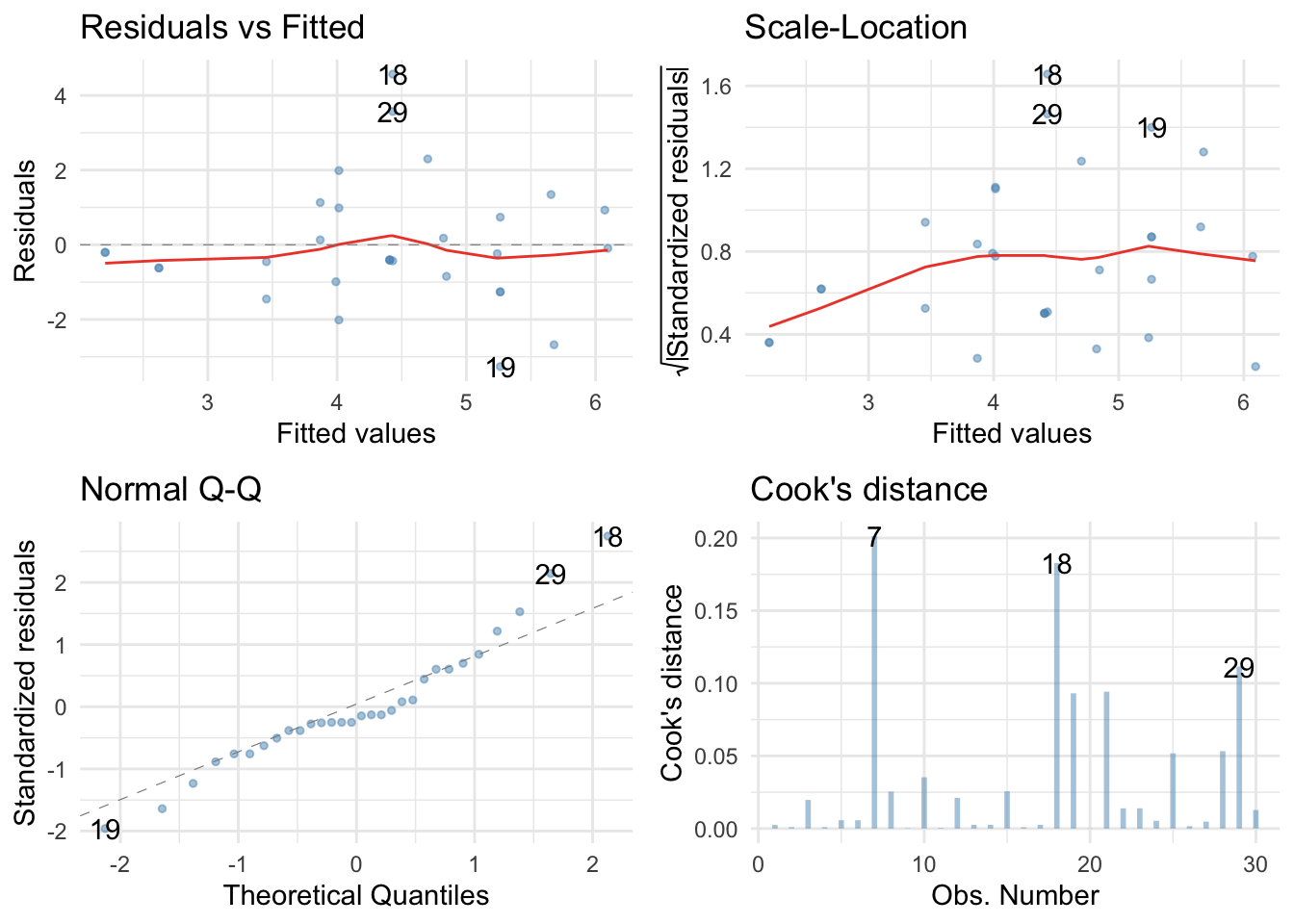
Residual plots:

ggplot2::autoplot(pupluv_lm,
                  which = c(1, 3, 2, 4),
                  colour = "#5c97bf",
                  smooth.colour = "#ef4836",
                  alpha = 0.5,
                  size = 1) + 
  theme_minimal()

robust model

Robust parameter estimates:

pupluv_rob <- robust::lmRob(happiness ~ puppy_love + dose, data = pupluv_tib)
summary(pupluv_rob)

## 
## Call:
## robust::lmRob(formula = happiness ~ puppy_love + dose, data = pupluv_tib)
## 
## Residuals:
##      Min       1Q   Median       3Q      Max 
## -2.34090 -0.34090  0.02081  0.89243  5.92569 
## 
## Coefficients:
##                   Estimate Std. Error t value Pr(>|t|)
## (Intercept)         2.1260     2.2616   0.940    0.356
## puppy_love          0.6333     0.5824   1.087    0.287
## dosepuppy_vs_none   1.6276     1.8641   0.873    0.391
## doseshort_vs_long  -0.4549     2.8052  -0.162    0.872
## 
## Residual standard error: 1.174 on 26 degrees of freedom
## Multiple R-Squared: 0.3901 
## 
## Test for Bias:
##             statistic p-value
## M-estimate     -5.868  1.0000
## LS-estimate     5.659  0.2261

Heteroscedasticity consistent standard errors:

parameters::model_parameters(pupluv_lm, robust = TRUE, vcov.type = "HC4", digits = 3)

Parameter	Coefficient	SE	CI_low	CI_high	t	df_error	p
(Intercept)	3.1260421	0.5920314	1.9091042	4.3429800	5.2801968	26	0.0000161
puppy_love	0.4160421	0.1985744	0.0078667	0.8242175	2.0951451	26	0.0460462
dosepuppy_vs_none	2.0052807	0.5157237	0.9451954	3.0653660	3.8882848	26	0.0006252
doseshort_vs_long	0.4392012	0.7399362	-1.0817594	1.9601619	0.5935663	26	0.5579313

Bootstrap parameters

parameters::bootstrap_parameters(pupluv_lm)

Parameter	Coefficient	CI_low	CI_high	p
(Intercept)	3.1893353	2.1168995	4.5143321	0.0000000
puppy_love	0.3954619	-0.0679983	0.7063347	0.0739261
dosepuppy_vs_none	1.9937821	0.8865644	3.0162401	0.0039960
doseshort_vs_long	0.3637506	-0.8214466	1.8375369	0.5954046

Bayes factors

pupcov_bf <-  BayesFactor::lmBF(formula = happiness ~ puppy_love, data = pupluv_tib, rscaleFixed = "medium", rscaleCont = "medium")
pupcov_bf

## Bayes factor analysis
## --------------
## [1] puppy_love : 0.6778239 ±0%
## 
## Against denominator:
##   Intercept only 
## ---
## Bayes factor type: BFlinearModel, JZS

pup_bf <-  BayesFactor::lmBF(formula = happiness ~ puppy_love + dose, data = pupluv_tib, rscaleCont = "medium", rscaleFixed = "medium")
pup_bf

## Bayes factor analysis
## --------------
## [1] puppy_love + dose : 1.431258 ±0.7%
## 
## Against denominator:
##   Intercept only 
## ---
## Bayes factor type: BFlinearModel, JZS

pup_bf/pupcov_bf

## Bayes factor analysis
## --------------
## [1] puppy_love + dose : 2.111548 ±0.7%
## 
## Against denominator:
##   happiness ~ puppy_love 
## ---
## Bayes factor type: BFlinearModel, JZS

Effect sizes

car::Anova(pupluv_lm, type = 3) %>% 
  effectsize::eta_squared(., ci = 0.95)

	Parameter	Eta_Sq_partial	CI	CI_low	CI_high
2	puppy_love	0.1601709	0.95	0	0.4108051
3	dose	0.2416256	0.95	0	0.4733256

Without a pipe:

pupluv_aov <- car::Anova(pupluv_lm, type = 3)
effectsize::omega_squared(pupluv_aov, ci = 0.95)

	Parameter	Omega_Sq_partial	CI	CI_low	CI_high
2	puppy_love	0.1165735	0.95	-0.0370370	0.3795428
3	dose	0.1731860	0.95	-0.0740741	0.4242189

Last updated on Aug 21, 2020