R code Chapter 11

This document contains abridged sections from Discovering Statistics Using R and RStudio by Andy Field so there are some copyright considerations. You can use this material for teaching and non-profit activities but please do not meddle with it or claim it as your own work. See the full license terms at the bottom of the page.
Load packages
Remember to load the tidyverse:
library(tidyverse)
Load the data
You can enter the data manually (for practice) with this code:
puppy_tib <- tibble::tibble(
  id = c("25hto3", "121118", "t54p42", "s6u853", "tcs14p", "oum4t7", "kfl7lq", "2gi51b", "d3j771", "eu23ns", "b343ey", "5nvg7h", "5ta11l", "82e7va", "667x5j"),
  dose = gl(3, 5, labels = c("No puppies", "15 mins", "30 mins")),
  happiness = c(3, 2, 1, 1, 4, 5, 2, 4, 2, 3, 7, 4, 5, 3, 6)
)
Alternatively, load it from the discover package. Remember to install the package with library(discovr). After which you can load data into a tibble by executing:
name_of_tib <- discovr::name_of_data
For example, execute these lines to create the tibbles referred to in the chapter:
puppy_tib <- discovr::puppies
If you want to read the file from the CSV (again, good practice) and you have set up your project folder as I suggest in Chapter 1, then the general format of the code you would use is:
tibble_name <- here::here("../data/name_of_file.csv") %>%
  readr::read_csv() %>%
  dplyr::mutate(
    ...
    code to convert character variables to factors
    ...
  )
In which you’d replace tibble_name with the name you want to assign to the tibble and change name_of_file.csv to the name of the file that you’re trying to load. You can use mutate to convert categorical variables to factors. For example, for the invisibility_cloak data you would load it by executing:
puppy_tib <- here::here("data/puppies.csv") %>%
  readr::read_csv() %>%
  dplyr::mutate(
    dose = forcats::as_factor(dose)
  )
A good idea to check that the levels of dose are in the order Control, 15 minutes, 30 minutes by executing:
levels(puppy_tib$dose)
## [1] "No puppies" "15 mins" "30 mins"
If they’re not in the correct order then:
puppy_tib <- puppy_tib %>%
  dplyr::mutate(
    dose = forcats::fct_relevel(dose, "No puppies", "15 mins", "30 mins")
  )
Self-test
puppy_tib <- puppy_tib %>%
  dplyr::mutate(
    dummy1 = ifelse(dose == "30 mins", 1, 0),
    dummy2 = ifelse(dose == "15 mins", 1, 0)
  )

puppy_lm <- lm(happiness ~ dummy1 + dummy2, data = puppy_tib)
broom::glance(puppy_lm)
## # A tibble: 1 x 12
##   r.squared adj.r.squared sigma statistic p.value    df logLik   AIC   BIC
##       <dbl>         <dbl> <dbl>     <dbl>   <dbl> <dbl>  <dbl> <dbl> <dbl>
## 1     0.460         0.370  1.40      5.12  0.0247     2  -24.7  57.4  60.2
## # … with 3 more variables: deviance <dbl>, df.residual <int>, nobs <int>
broom::tidy(puppy_lm, conf.int = TRUE)
## # A tibble: 3 x 7
##   term        estimate std.error statistic p.value conf.low conf.high
##   <chr>          <dbl>     <dbl>     <dbl>   <dbl>    <dbl>     <dbl>
## 1 (Intercept)     2.20     0.627      3.51 0.00432    0.834      3.57
## 2 dummy1          2.8      0.887      3.16 0.00827    0.868      4.73
## 3 dummy2          1.       0.887      1.13 0.282     -0.932      2.93
Self-test
Create the dummy variables:
puppy_tib <- puppy_tib %>%
  dplyr::mutate(
    contrast1 = ifelse(dose == "No puppies", -2/3, 1/3),
    contrast2 = dplyr::case_when(
      dose == "No puppies" ~ 0,
      dose == "15 mins" ~ -0.5,
      dose == "30 mins" ~ 0.5)
  )
Alternatively using nested ifelse() statements:
puppy_tib <- puppy_tib %>%
  dplyr::mutate(
    contrast1 = ifelse(dose == "No puppies", -2/3, 1/3),
    contrast2 = ifelse(dose == "No puppies", 0,
                    ifelse(dose == "15 mins", -0.5, 0.5))
  )
Fit and inspect the model:
puppy_con_lm <- lm(happiness ~ contrast1 + contrast2, data = puppy_tib)
broom::glance(puppy_con_lm)
## # A tibble: 1 x 12
##   r.squared adj.r.squared sigma statistic p.value    df logLik   AIC   BIC
##       <dbl>         <dbl> <dbl>     <dbl>   <dbl> <dbl>  <dbl> <dbl> <dbl>
## 1     0.460         0.370  1.40      5.12  0.0247     2  -24.7  57.4  60.2
## # … with 3 more variables: deviance <dbl>, df.residual <int>, nobs <int>
broom::tidy(puppy_con_lm, conf.int = TRUE) %>%
  dplyr::mutate(
    dplyr::across(where(is.numeric), ~round(., 3))
  )
## # A tibble: 3 x 7
##   term        estimate std.error statistic p.value conf.low conf.high
##   <chr>          <dbl>     <dbl>     <dbl>   <dbl>    <dbl>     <dbl>
## 1 (Intercept)     3.47     0.362      9.57   0        2.68       4.26
## 2 contrast1       1.9      0.768      2.47   0.029    0.226      3.57
## 3 contrast2       1.8      0.887      2.03   0.065   -0.132      3.73
Summary statistics and plot
A violin plot
ggplot2::ggplot(puppy_tib, aes(dose, happiness)) +
  geom_violin() +
  stat_summary(fun.data = "mean_cl_boot") +
  labs(x = "Dose of puppies", y = "Happiness (0-10)") +
  scale_y_continuous(breaks = 1:7) +
  theme_minimal()
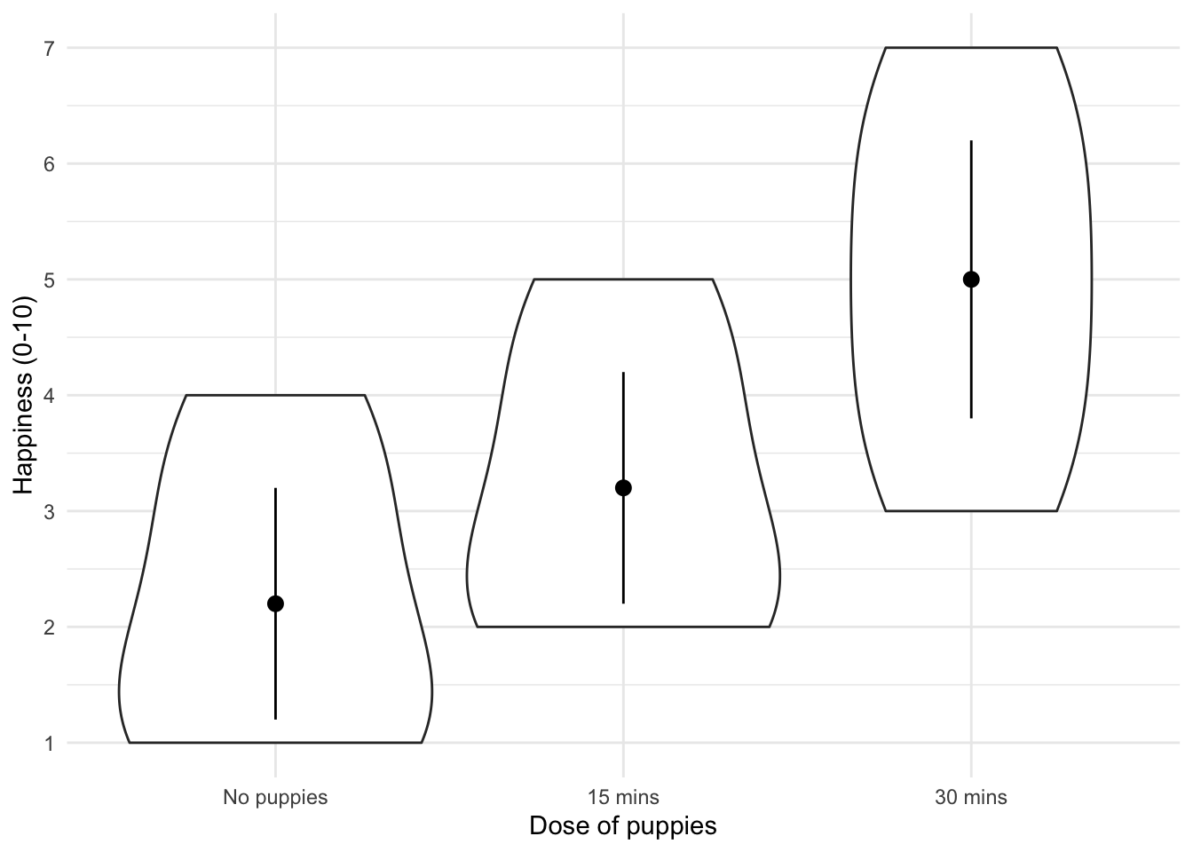
Summary statistics
puppy_tib %>%
  dplyr::group_by(dose) %>%
  dplyr::summarize(
    valid_cases = sum(!is.na(happiness)),
    min = min(happiness, na.rm = TRUE),
    max = max(happiness, na.rm = TRUE),
    median = median(happiness, na.rm = TRUE),
    mean = mean(happiness, na.rm = TRUE),
    sd = sd(happiness, na.rm = TRUE),
    `95% CI lower` = mean_cl_normal(happiness)$ymin,
    `95% CI upper` = mean_cl_normal(happiness)$ymax
  ) %>%
  dplyr::mutate(
    dplyr::across(where(is.numeric), ~round(., 2))
  )
## # A tibble: 3 x 9
##   dose  valid_cases   min   max median  mean    sd `95% CI lower` `95% CI upper`
##   <fct>       <dbl> <dbl> <dbl>  <dbl> <dbl> <dbl>          <dbl>          <dbl>
## 1 No p…           5     1     4      2   2.2  1.3           0.580           3.82
## 2 15 m…           5     2     5      3   3.2  1.3           1.58            4.82
## 3 30 m…           5     3     7      5   5    1.58          3.04            6.96
Set contrasts
This code sets a treatment contrast to the variable dose that compares each category to the last.
contrasts(puppy_tib$dose) <- contr.treatment(3, base = 3)
We can look at the contrast by executing:
contrasts(puppy_tib$dose)
##            1 2
## No puppies 1 0
## 15 mins    0 1
## 30 mins    0 0
Let’s set the actual planned contrasts from the chapter:
puppy_vs_none <- c(-2/3, 1/3, 1/3)
short_vs_long <- c(0, -1/2, 1/2)

contrasts(puppy_tib$dose) <- cbind(puppy_vs_none, short_vs_long)
contrasts(puppy_tib$dose) # check the contrasts are set correctly
##            puppy_vs_none short_vs_long
## No puppies    -0.6666667           0.0
## 15 mins        0.3333333          -0.5
## 30 mins        0.3333333           0.5
Fit the model
Assumptions met
puppy_lm <- lm(happiness ~ dose, data = puppy_tib, na.action = na.exclude)

anova(puppy_lm) %>%
  parameters::parameters(., omega_squared = "raw")
## Parameter | Sum_Squares | df | Mean_Square |    F |     p | Omega_Sq (partial)
## ------------------------------------------------------------------------------
## dose      |       20.13 |  2 |       10.07 | 5.12 | 0.025 |               0.35
## Residuals |       23.60 | 12 |        1.97 |      |       |
broom::tidy(puppy_lm, conf.int = TRUE) %>%
  dplyr::mutate(
    dplyr::across(where(is.numeric), ~round(., 3))
  )
## # A tibble: 3 x 7
##   term              estimate std.error statistic p.value conf.low conf.high
##   <chr>                <dbl>     <dbl>     <dbl>   <dbl>    <dbl>     <dbl>
## 1 (Intercept)           3.47     0.362      9.57   0        2.68       4.26
## 2 dosepuppy_vs_none     1.9      0.768      2.47   0.029    0.226      3.57
## 3 doseshort_vs_long     1.8      0.887      2.03   0.065   -0.132      3.73
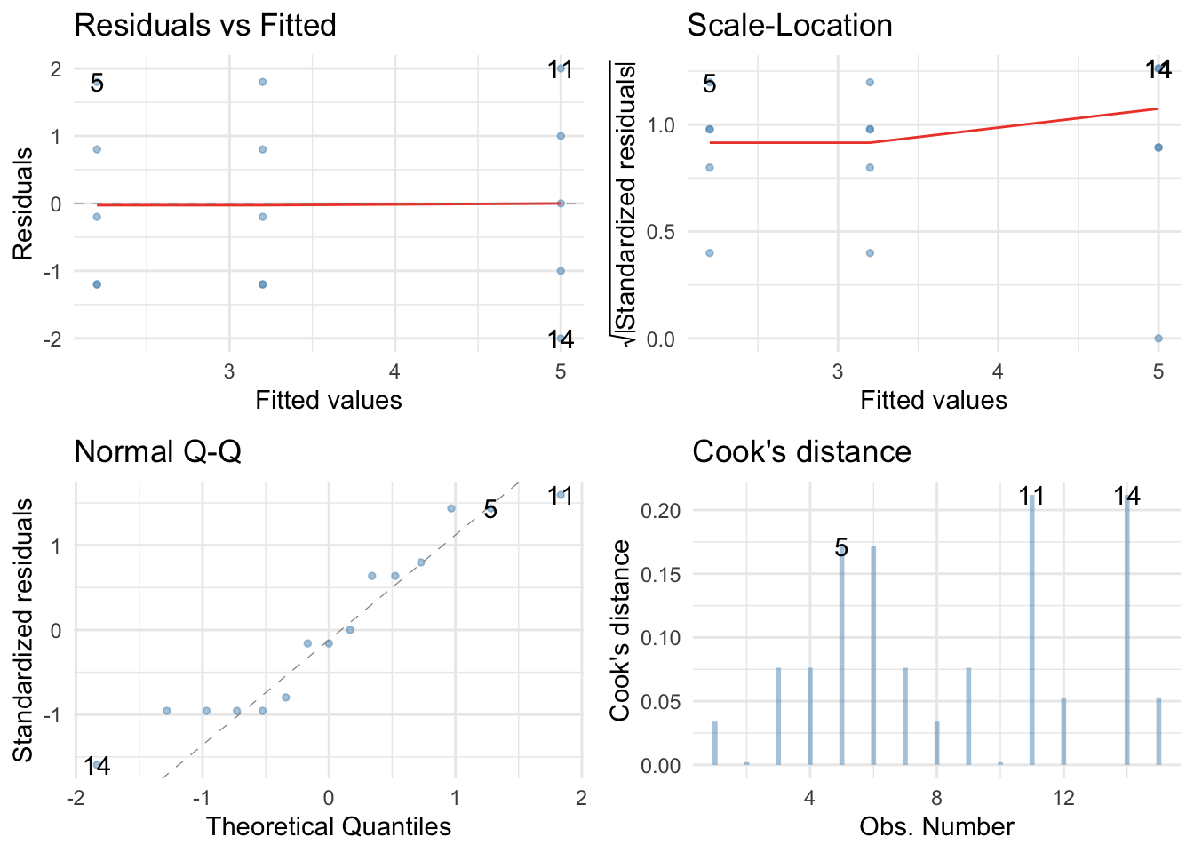
Residual plots:
ggplot2::autoplot(puppy_lm,
                  which = c(1, 3, 2, 4),
                  colour = "#5c97bf",
                  smooth.colour = "#ef4836",
                  alpha = 0.5,
                  size = 1) +
  theme_minimal()
Post hoc tests
modelbased::estimate_contrasts(puppy_lm)
## Level1     |  Level2 | Difference |   SE |         95% CI |     t | df |     p | Difference (std.)
## --------------------------------------------------------------------------------------------------
## 15 mins    | 30 mins |      -1.80 | 0.89 | [-4.27,  0.67] | -2.03 | 12 | 0.130 |             -1.02
## No puppies | 15 mins |      -1.00 | 0.89 | [-3.47,  1.47] | -1.13 | 12 | 0.282 |             -0.57
## No puppies | 30 mins |      -2.80 | 0.89 | [-5.27, -0.33] | -3.16 | 12 | 0.025 |             -1.58
Bonferroni:
modelbased::estimate_contrasts(puppy_lm, adjust = "bonferroni")
## Level1     |  Level2 | Difference |   SE |         95% CI |     t | df |     p | Difference (std.)
## --------------------------------------------------------------------------------------------------
## 15 mins    | 30 mins |      -1.80 | 0.89 | [-4.27,  0.67] | -2.03 | 12 | 0.196 |             -1.02
## No puppies | 15 mins |      -1.00 | 0.89 | [-3.47,  1.47] | -1.13 | 12 | 0.845 |             -0.57
## No puppies | 30 mins |      -2.80 | 0.89 | [-5.27, -0.33] | -3.16 | 12 | 0.025 |             -1.58
Trend analysis
contrasts(puppy_tib$dose) <- contr.poly(3)

puppy_trend <- lm(happiness ~ dose, data = puppy_tib, na.action = na.exclude)

broom::tidy(puppy_trend, conf.int = TRUE) %>%
  dplyr::mutate(
    dplyr::across(where(is.numeric), ~round(., 3))
  )
## # A tibble: 3 x 7
##   term        estimate std.error statistic p.value conf.low conf.high
##   <chr>          <dbl>     <dbl>     <dbl>   <dbl>    <dbl>     <dbl>
## 1 (Intercept)    3.47      0.362     9.57    0        2.68       4.26
## 2 dose.L         1.98      0.627     3.16    0.008    0.613      3.35
## 3 dose.Q         0.327     0.627     0.521   0.612   -1.04       1.69
robust model
Because of doing the trend analysis above, where we reset the contrast for dose, let’s set it back to how it was for the main example:
contrasts(puppy_tib$dose) <- cbind(puppy_vs_none, short_vs_long)
Robust F
oneway.test(happiness ~ dose, data = puppy_tib)
##
## 	One-way analysis of means (not assuming equal variances)
##
## data:  happiness and dose
## F = 4.3205, num df = 2.0000, denom df = 7.9434, p-value = 0.05374
Robust parameter estimates:
puppy_rob <- robust::lmRob(happiness ~ dose, data = puppy_tib)
summary(puppy_rob)
##
## Call:
## robust::lmRob(formula = happiness ~ dose, data = puppy_tib)
##
## Residuals:
##    Min     1Q Median     3Q    Max
##   -2.0   -1.2   -0.2    0.9    2.0
##
## Coefficients:
##                   Estimate Std. Error t value Pr(>|t|)
## (Intercept)         3.4667     0.3651   9.494 6.26e-07 ***
## dosepuppy_vs_none   1.9000     0.7746   2.453   0.0304 *
## doseshort_vs_long   1.8000     0.8944   2.012   0.0672 .
## ---
## Signif. codes:  0 '***' 0.001 '**' 0.01 '*' 0.05 '.' 0.1 ' ' 1
##
## Residual standard error: 1.867 on 12 degrees of freedom
## Multiple R-Squared: 0.4604
##
## Test for Bias:
##             statistic p-value
## M-estimate   -0.04843  1.0000
## LS-estimate   1.38600  0.7088
Heteroscedasticity consistent standard errors:
parameters::model_parameters(puppy_lm, robust = TRUE, vcov.type = "HC4", digits = 3)
## Parameter         | Coefficient |    SE |        95% CI |     t | df |      p
## -----------------------------------------------------------------------------
## (Intercept)       |       3.467 | 0.405 | [ 2.58, 4.35] | 8.563 | 12 | < .001
## dosepuppy_vs_none |       1.900 | 0.829 | [ 0.09, 3.71] | 2.291 | 12 | 0.041
## doseshort_vs_long |       1.800 | 1.025 | [-0.43, 4.03] | 1.757 | 12 | 0.104
WRS2 package
WRS2::t1way(happiness ~ dose, data = puppy_tib, nboot = 1000)
## Call:
## WRS2::t1way(formula = happiness ~ dose, data = puppy_tib, nboot = 1000)
##
## Test statistic: F = 3
## Degrees of freedom 1: 2
## Degrees of freedom 2: 4
## p-value: 0.16
##
## Explanatory measure of effect size: 0.79
## Bootstrap CI: [0.43; 1.35]
WRS2::lincon(happiness ~ dose, data = puppy_tib)
## Call:
## WRS2::lincon(formula = happiness ~ dose, data = puppy_tib)
##
##                        psihat ci.lower ci.upper p.value
## No puppies vs. 15 mins     -1 -5.31858  3.31858 0.43533
## No puppies vs. 30 mins     -3 -7.31858  1.31858 0.18051
## 15 mins vs. 30 mins        -2 -6.31858  2.31858 0.31660
WRS2::t1waybt(happiness ~ dose, data = puppy_tib, nboot = 1000)
## Call:
## WRS2::t1waybt(formula = happiness ~ dose, data = puppy_tib, nboot = 1000)
##
## Effective number of bootstrap samples was 606.
##
## Test statistic: 3
## p-value: 0.07261
## Variance explained: 0.623
## Effect size: 0.789
WRS2::mcppb20(happiness ~ dose, data = puppy_tib, nboot = 1000)
## Call:
## WRS2::mcppb20(formula = happiness ~ dose, data = puppy_tib, nboot = 1000)
##
##                        psihat ci.lower ci.upper p-value
## No puppies vs. 15 mins     -1 -3.33333  1.00000   0.288
## No puppies vs. 30 mins     -3 -5.33333 -0.33333   0.005
## 15 mins vs. 30 mins        -2 -4.33333  0.66667   0.079
Self-test
WRS2::t1way(happiness ~ dose, data = puppy_tib, tr = 0.1, nboot = 1000)
## Call:
## WRS2::t1way(formula = happiness ~ dose, data = puppy_tib, tr = 0.1,
##     nboot = 1000)
##
## Test statistic: F = 4.3205
## Degrees of freedom 1: 2
## Degrees of freedom 2: 7.94
## p-value: 0.05374
##
## Explanatory measure of effect size: 0.71
## Bootstrap CI: [0.5; 0.95]
WRS2::lincon(happiness ~ dose, data = puppy_tib, tr = 0.1)
## Call:
## WRS2::lincon(formula = happiness ~ dose, data = puppy_tib, tr = 0.1)
##
##                        psihat ci.lower ci.upper p.value
## No puppies vs. 15 mins   -1.0 -3.44088  1.44088 0.25985
## No puppies vs. 30 mins   -2.8 -5.53616 -0.06384 0.04915
## 15 mins vs. 30 mins      -1.8 -4.53616  0.93616 0.17289
Bayes factors
puppy_bf <-  BayesFactor::lmBF(formula = happiness ~ dose, data = puppy_tib, rscaleFixed = "medium")
puppy_bf
## Bayes factor analysis
## --------------
## [1] dose : 3.070605 ±0.01%
##
## Against denominator:
##   Intercept only
## ---
## Bayes factor type: BFlinearModel, JZS