R code Chapter 9

This document contains abridged sections from Discovering Statistics Using R and RStudio by Andy Field so there are some copyright considerations. You can use this material for teaching and non-profit activities but please do not meddle with it or claim it as your own work. See the full license terms at the bottom of the page.
Load packages
Remember to load the tidyverse:
library(tidyverse)
Load the data
Remember to install the package for the book with library(discovr). After which you can load data into a tibble by executing:
name_of_tib <- discovr::name_of_data
For example, execute these lines to create the tibbles referred to in the chapter:
cloak_tib <- discovr::invisibility_cloak
cloak_rm_tib <- discovr::invisibility_rm
If you want to read the file from the CSV and you have set up your project folder as I suggest in Chapter 1, then the general format of the code you would use is:
tibble_name <- here::here("../data/name_of_file.csv") %>%
  readr::read_csv() %>%
  dplyr::mutate(
    ...
    code to convert character variables to factors
    ...
  )
In which you’d replace tibble_name with the name you want to assign to the tibble and change name_of_file.csv to the name of the file that you’re trying to load. You can use mutate to convert categorical variables to factors. For example, for the invisibility_cloak data you would load it by executing:
library(here)

cloak_tib <- here::here("data/invisibility.csv") %>%
  readr::read_csv() %>%
  dplyr::mutate(
    cloak = forcats::as_factor(cloak)
  )
Entering data
You were given the task to enter the data, there are several ways to do this, but here’s one of them:
cloak_tib <- tibble::tibble(
    id = c("Kiara", "Anupama", "Collin", "Ian", "Vanessa", "Darrell", "Tyler", "Steven", "Katheryn", "Kirkpatrick", "Melissa", "Kinaana", "Shajee'a", "Sage", "Jorge", "Conan","Tamara","Man", "Joseph", "Israa", "Kathryn", "Luis", "Devante", "Jerry"),
    cloak = gl(2, 12, labels = c("No cloak", "Cloak")),
    mischief = c(3, 1, 5, 4, 6, 4, 6, 2, 0, 5, 4, 5, 4, 3, 6, 6, 8, 5, 5, 4, 2, 5, 7, 5)
  )
Descriptive statistics
cloak_tib %>%
  dplyr::group_by(cloak) %>%
  dplyr::summarize(
    n = n(),
    mean = mean(mischief),
    sd = sd(mischief),
    ci_lower = ggplot2::mean_cl_normal(mischief)$ymin,
    ci_upper = ggplot2::mean_cl_normal(mischief)$ymax,
    iqr = IQR(mischief),
    skew = moments::skewness(mischief),
    kurtosis = moments::kurtosis(mischief)
  )
## # A tibble: 2 x 9
##   cloak        n  mean    sd ci_lower ci_upper   iqr   skew kurtosis
##   <fct>    <int> <dbl> <dbl>    <dbl>    <dbl> <dbl>  <dbl>    <dbl>
## 1 No cloak    12  3.75  1.91     2.53     4.97  2.25 -0.687     2.39
## 2 Cloak       12  5     1.65     3.95     6.05  2     0         2.64
cloak_lm <- lm(mischief ~ cloak, data = cloak_tib)
summary(cloak_lm)
##
## Call:
## lm(formula = mischief ~ cloak, data = cloak_tib)
##
## Residuals:
##    Min     1Q Median     3Q    Max
## -3.750 -1.000  0.125  1.250  3.000
##
## Coefficients:
##             Estimate Std. Error t value Pr(>|t|)
## (Intercept)   3.7500     0.5158   7.270 2.79e-07 ***
## cloakCloak    1.2500     0.7295   1.713    0.101
## ---
## Signif. codes:  0 '***' 0.001 '**' 0.01 '*' 0.05 '.' 0.1 ' ' 1
##
## Residual standard error: 1.787 on 22 degrees of freedom
## Multiple R-squared:  0.1177,	Adjusted R-squared:  0.07764
## F-statistic: 2.936 on 1 and 22 DF,  p-value: 0.1007
t-test from summary data
t_from_means <- function(m1, m2, sd1, sd2, n1, n2){
  df <- n1 + n2 - 2
	poolvar <- (((n1-1)*sd1^2)+((n2-1)*sd2^2))/df
	t <- (m1-m2)/sqrt(poolvar*((1/n1)+(1/n2)))
	sig <- 2*(1-(pt(abs(t),df)))
	paste0("t(df = ", df, ") = ", round(t, 3), ", p = ", round(sig, 5))
}

t_from_means(m1 = 5, m2 = 3.75, sd1 = 1.651, sd2 = 1.913, n1 = 12, n2 = 12)
## [1] "t(df = 22) = 1.714, p = 0.10066"
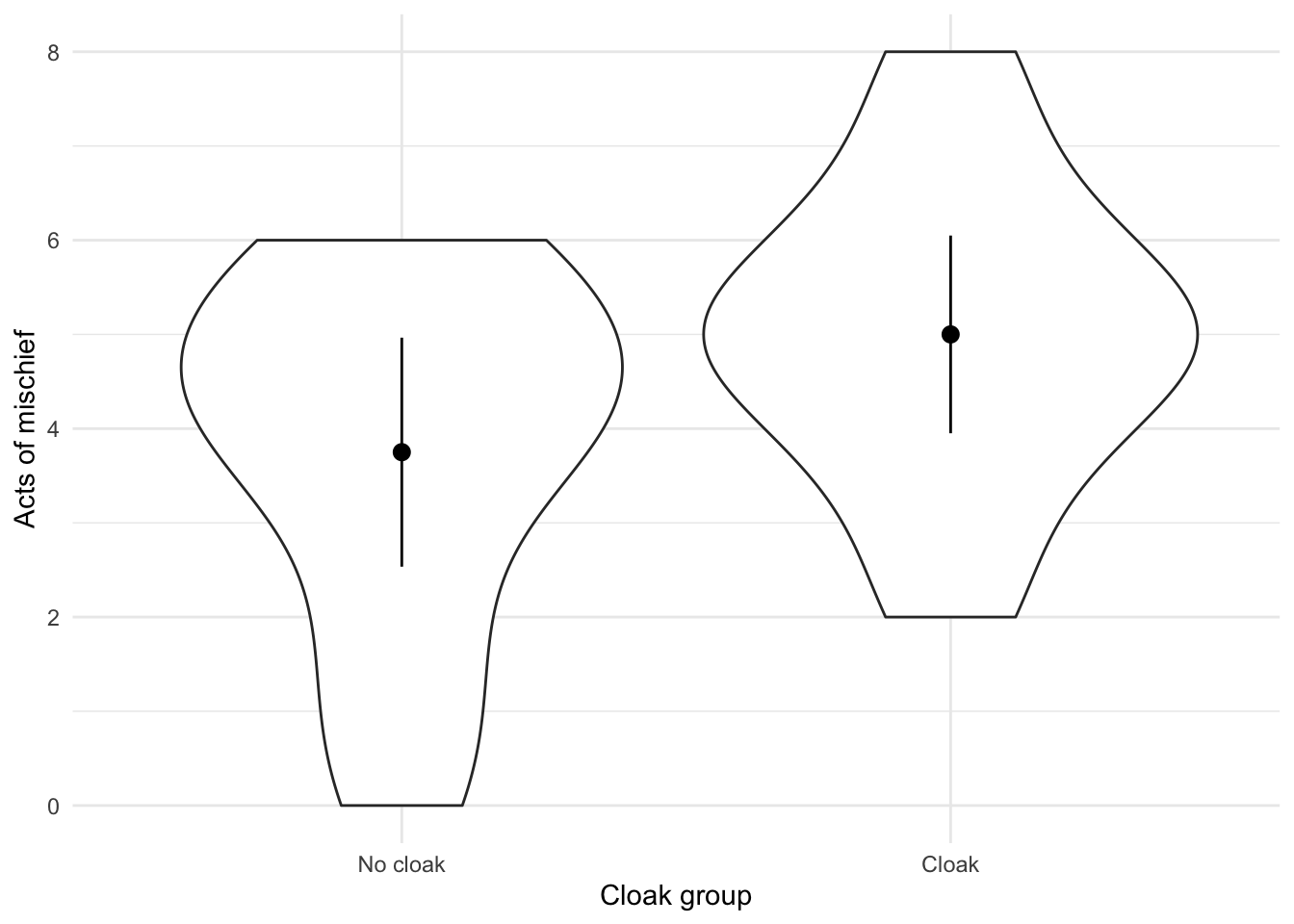
Error bar plot
ggplot2::ggplot(cloak_tib, aes(cloak, mischief)) +
  geom_violin() +
  stat_summary(fun.data = "mean_cl_normal") +
  labs(x = "Cloak group", y = "Acts of mischief") +
  theme_minimal()
Independent t-test
cloak_mod <- t.test(mischief ~ cloak, data = cloak_tib)
cloak_mod
##
## 	Welch Two Sample t-test
##
## data:  mischief by cloak
## t = -1.7135, df = 21.541, p-value = 0.101
## alternative hypothesis: true difference in means is not equal to 0
## 95 percent confidence interval:
##  -2.764798  0.264798
## sample estimates:
## mean in group No cloak    mean in group Cloak
##                   3.75                   5.00
Robust tests
yuen()
WRS2::yuen(mischief ~ cloak, data = cloak_tib)
## Call:
## WRS2::yuen(formula = mischief ~ cloak, data = cloak_tib)
##
## Test statistic: 1.4771 (df = 12.26), p-value = 0.16487
##
## Trimmed mean difference:  -1
## 95 percent confidence interval:
## -2.4716     0.4716
##
## Explanatory measure of effect size: 0.4
WRS2::yuen(mischief ~ cloak, data = cloak_tib, tr = 0.1)
## Call:
## WRS2::yuen(formula = mischief ~ cloak, data = cloak_tib, tr = 0.1)
##
## Test statistic: 1.4245 (df = 16.9), p-value = 0.1725
##
## Trimmed mean difference:  -1.1
## 95 percent confidence interval:
## -2.7299     0.5299
##
## Explanatory measure of effect size: 0.45
yuenbt()
WRS2::yuenbt(mischief ~ cloak, data = cloak_tib, nboot = 1000, side = TRUE)
## Call:
## WRS2::yuenbt(formula = mischief ~ cloak, data = cloak_tib, nboot = 1000,
##     side = TRUE)
##
## Test statistic: -1.3607 (df = NA), p-value = 0.172
##
## Trimmed mean difference:  -1
## 95 percent confidence interval:
## -2.5     0.5
pb2gen()
WRS2::pb2gen(mischief ~ cloak, data = cloak_tib, nboot = 1000)
## Call:
## WRS2::pb2gen(formula = mischief ~ cloak, data = cloak_tib, nboot = 1000)
##
## Test statistic: -0.9091, p-value = 0.244
## 95% confidence interval:
## -2.6667    0.5333
Bayes factor for indepedent means
cloak_bf <- BayesFactor::ttestBF(formula = mischief ~ cloak, data = cloak_tib)
cloak_bf
## Bayes factor analysis
## --------------
## [1] Alt., r=0.707 : 1.050917 ±0%
##
## Against denominator:
##   Null, mu1-mu2 = 0
## ---
## Bayes factor type: BFindepSample, JZS
BayesFactor::posterior(cloak_bf, iterations = 1000) %>%
  summary()
##
## Iterations = 1:1000
## Thinning interval = 1
## Number of chains = 1
## Sample size per chain = 1000
##
## 1. Empirical mean and standard deviation for each variable,
##    plus standard error of the mean:
##
##                            Mean      SD Naive SE Time-series SE
## mu                       4.3612  0.3875  0.01225        0.01225
## beta (No cloak - Cloak) -0.9176  0.6686  0.02114        0.02490
## sig2                     3.4620  1.1013  0.03482        0.03735
## delta                   -0.5140  0.3762  0.01190        0.01398
## g                        3.2559 22.9528  0.72583        0.72583
##
## 2. Quantiles for each variable:
##
##                             2.5%     25%     50%     75%   97.5%
## mu                       3.58203  4.0980  4.3776  4.6234  5.0966
## beta (No cloak - Cloak) -2.27040 -1.3528 -0.9114 -0.4677  0.3839
## sig2                     1.85419  2.6661  3.2815  4.0793  6.0981
## delta                   -1.27113 -0.7624 -0.5017 -0.2538  0.1734
## g                        0.09155  0.2704  0.5851  1.4440 15.7681
1/cloak_bf
## Bayes factor analysis
## --------------
## [1] Null, mu1-mu2=0 : 0.9515501 ±0%
##
## Against denominator:
##   Alternative, r = 0.707106781186548, mu =/= 0
## ---
## Bayes factor type: BFindepSample, JZS
Effect sizes
effectsize::t_to_r(t = cloak_mod$statistic, df_error = cloak_mod$parameter)
##     r |        95% CI
## ---------------------
## -0.35 | [-0.63, 0.07]
effectsize::cohens_d(mischief ~ cloak, data = cloak_tib)
## Cohen's d |        95% CI
## -------------------------
##     -0.70 | [-1.52, 0.13]
effectsize::hedges_g(mischief ~ cloak, data = cloak_tib)
## Hedge's g |        95% CI
## -------------------------
##     -0.68 | [-1.47, 0.13]
effectsize::glass_delta(mischief ~ cloak, data = cloak_tib)
## Glass' delta |        95% CI
## ----------------------------
##        -0.76 | [-1.58, 0.08]
r_from_t <- function(t, df, digits = 5){
  r <- sqrt(t^2/(t^2+df))
  r <- round(r, digits)
  return(paste0("r = ", r))
}

r_from_t(t = cloak_mod$statistic, df = cloak_mod$parameter)
## [1] "r = 0.34633"
r_from_t(t = cloak_mod$statistic, df = cloak_mod$parameter, digits = 2)
## [1] "r = 0.35"
Entering data for related means
cloak_rm_tib <- tibble::tibble(
    id = rep(c("Alia", " Elisia", "Dominika", "Noah", "Haashid", "Zainab", "Reyna", "Victoria", "Najaat", "Jordyn", "Zaki", "Rajohn"), 2),
    cloak = gl(2, 12, labels = c("No cloak", "Cloak")),
    mischief = c(3, 1, 5, 4, 6, 4, 6, 2, 0, 5, 4, 5, 4, 3, 6, 6, 8, 5, 5, 4, 2, 5, 7, 5)
  )
Or load it from the package:
cloak_rm_tib <- discovr::invisibility_rm
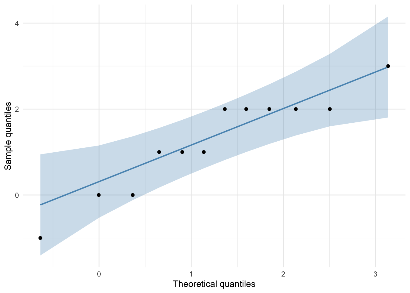
Plot of the differences between scores:
cloak_rm_tib %>%
  tidyr::pivot_wider(
    id_cols = id,
    values_from = mischief,
    names_from = cloak
    ) %>%
  dplyr::mutate(
    diff = Cloak - `No cloak`
  ) %>%  ggplot2::ggplot(., aes(sample = diff)) +
    qqplotr::stat_qq_band(fill = "#5c97bf", alpha = 0.3) +
    qqplotr::stat_qq_line(colour = "#5c97bf") +
    qqplotr::stat_qq_point() +
    labs(x = "Theoretical quantiles", y = "Sample quantiles") +
    theme_minimal()
Paired t-test
cloak_rm_mod <- t.test(mischief ~ cloak, data = cloak_rm_tib, paired = TRUE)
cloak_rm_mod
##
## 	Paired t-test
##
## data:  mischief by cloak
## t = -3.8044, df = 11, p-value = 0.002921
## alternative hypothesis: true difference in means is not equal to 0
## 95 percent confidence interval:
##  -1.9731653 -0.5268347
## sample estimates:
## mean of the differences
##                   -1.25
Showing that order matters:
cloak_rm_tib %>%
  dplyr::sample_n(24) %>%
  t.test(mischief ~ cloak, data = ., paired = TRUE)
##
## 	Paired t-test
##
## data:  mischief by cloak
## t = -1.5646, df = 11, p-value = 0.146
## alternative hypothesis: true difference in means is not equal to 0
## 95 percent confidence interval:
##  -3.0083896  0.5083896
## sample estimates:
## mean of the differences
##                   -1.25
Making sure that data are in the correct order by sorting by participant id:
cloak_rm_tib %>%
  dplyr::arrange(id) %>%
  t.test(mischief ~ cloak, data = ., paired = TRUE)
##
## 	Paired t-test
##
## data:  mischief by cloak
## t = -3.8044, df = 11, p-value = 0.002921
## alternative hypothesis: true difference in means is not equal to 0
## 95 percent confidence interval:
##  -1.9731653 -0.5268347
## sample estimates:
## mean of the differences
##                   -1.25
Robust tests of dependent means
yuend()
cloak_messy_tib <- cloak_rm_tib %>%
  tidyr::spread(value = mischief, key = cloak)

WRS2::yuend(cloak_messy_tib$Cloak, cloak_messy_tib$`No cloak`)
## Call:
## WRS2::yuend(x = cloak_messy_tib$Cloak, y = cloak_messy_tib$`No cloak`)
##
## Test statistic: 2.7027 (df = 7), p-value = 0.03052
##
## Trimmed mean difference:  1
## 95 percent confidence interval:
## 0.1251     1.8749
##
## Explanatory measure of effect size: 0.4
Bayes factor for depedent means
cloak_rm_bf <- BayesFactor::ttestBF(cloak_messy_tib$Cloak, cloak_messy_tib$`No cloak`, paired = TRUE, rscale = "medium")
cloak_rm_bf
## Bayes factor analysis
## --------------
## [1] Alt., r=0.707 : 16.28906 ±0%
##
## Against denominator:
##   Null, mu = 0
## ---
## Bayes factor type: BFoneSample, JZS
BayesFactor::posterior(cloak_rm_bf, iterations = 1000) %>%
  summary()
##
## Iterations = 1:1000
## Thinning interval = 1
## Number of chains = 1
## Sample size per chain = 1000
##
## 1. Empirical mean and standard deviation for each variable,
##    plus standard error of the mean:
##
##         Mean      SD Naive SE Time-series SE
## mu    1.1031  0.3614  0.01143        0.01291
## sig2  1.6357  0.8525  0.02696        0.03023
## delta 0.9317  0.3559  0.01125        0.01353
## g     5.3619 22.5048  0.71166        0.80593
##
## 2. Quantiles for each variable:
##
##         2.5%    25%    50%   75%  97.5%
## mu    0.3743 0.8698 1.1109 1.334  1.815
## sig2  0.6774 1.0835 1.4352 1.923  3.936
## delta 0.2623 0.6798 0.9290 1.170  1.605
## g     0.1447 0.4604 0.9867 2.546 42.049
1/cloak_rm_bf
## Bayes factor analysis
## --------------
## [1] Null, mu=0 : 0.06139091 ±0%
##
## Against denominator:
##   Alternative, r = 0.707106781186548, mu =/= 0
## ---
## Bayes factor type: BFoneSample, JZS
Effect sizes for dependent means
Do the same as for independent designs (see earlier). If you must, you can do this:
cloak_rm_tib %>%
  dplyr::arrange(id) %>%
  effectsize::cohens_d(mischief ~ cloak, data = ., paired = TRUE)
## Cohen's d |         95% CI
## --------------------------
##     -1.10 | [-1.89, -0.37]
cloak_rm_tib %>%
  dplyr::arrange(id) %>%
  effectsize::hedges_g(mischief ~ cloak, data = ., paired = TRUE)
## Hedge's g |         95% CI
## --------------------------
##     -1.02 | [-1.76, -0.35]
effectsize::t_to_r(t = cloak_mod$statistic, df_error = cloak_mod$parameter)
##     r |        95% CI
## ---------------------
## -0.35 | [-0.63, 0.07]