R code Chapter 8

This document contains abridged sections from Discovering Statistics Using R and RStudio by Andy Field so there are some copyright considerations. You can use this material for teaching and non-profit activities but please do not meddle with it or claim it as your own work. See the full license terms at the bottom of the page.
Load packages
Remember to load the tidyverse:
library(tidyverse)
Load the data
Remember to install the package for the book with library(discovr). After which you can load data into a tibble by executing:
name_of_tib <- discovr::name_of_data
For example, execute these lines to create the tibbles referred to in the chapter:
album_tib <- discovr::album_sales
df_tib <- discovr::df_beta
pub_tib <- discovr::pubs
If you want to read the file from the CSV and you have set up your project folder as I suggest in Chapter 1, then the general format of the code you would use is:
tibble_name <- here::here("../data/name_of_file.csv") %>%
  readr::read_csv() %>%
  dplyr::mutate(
    ...
    code to convert character variables to factors
    ...
  )
In which you’d replace tibble_name with the name you want to assign to the tibble and change name_of_file.csv to the name of the file that you’re trying to load. You can use mutate to convert categorical variables to factors. For example, for the album_sales data you would load it by executing:
library(here)

album_tib <- here::here("data/album_sales.csv") %>%
  readr::read_csv()
Self test on df_beta
Load the data and fit the model with all cases.
df_tib <- discovr::df_beta

df_lm <- df_tib %>%
  lm(y ~ x, data = .)

df_lm %>%
  broom::tidy()
## # A tibble: 2 x 5
##   term        estimate std.error statistic  p.value
##   <chr>          <dbl>     <dbl>     <dbl>    <dbl>
## 1 (Intercept)   29.0      0.992       29.2 1.58e-22
## 2 x             -0.903    0.0559     -16.2 9.90e-16
Fit the model with case 30 excluded.
df_tib %>%
  dplyr::filter(case != 30) %>%
  lm(y ~ x, data = .) %>%
  broom::tidy()
## # A tibble: 2 x 5
##   term        estimate std.error statistic p.value
##   <chr>          <dbl>     <dbl>     <dbl>   <dbl>
## 1 (Intercept)      31.  1.39e-15   2.24e16       0
## 2 x                -1   7.68e-17  -1.30e16       0
Other diagnostics (look at the values for case 30):
dfbeta(df_lm)
##      (Intercept)             x
## 1   0.0689655172 -6.674082e-03
## 2   0.0544297438 -5.469987e-03
## 3   0.0418250951 -4.399554e-03
## 4   0.0310406796 -3.454527e-03
## 5   0.0219815743 -2.627778e-03
## 6   0.0145669922 -1.913176e-03
## 7   0.0087287732 -1.305476e-03
## 8   0.0044101433 -8.002276e-04
## 9   0.0015647004 -3.936988e-04
## 10  0.0001555936 -8.281594e-05
## 11  0.0001548707  1.348874e-04
## 12  0.0015429718  2.613097e-04
## 13  0.0043083551  2.978126e-04
## 14  0.0084472431  2.452425e-04
## 15  0.0139634801  1.039465e-04
## 16  0.0208684978 -1.262208e-04
## 17  0.0291813853 -4.458955e-04
## 18  0.0389290660 -8.562111e-04
## 19  0.0501465823 -1.358811e-03
## 20  0.0628774973 -1.955867e-03
## 21  0.0771744204 -2.650110e-03
## 22  0.0930996714 -3.444865e-03
## 23  0.1107260986 -4.344093e-03
## 24  0.1301380733 -5.352453e-03
## 25  0.1514326877 -6.475366e-03
## 26  0.1747211896 -7.719099e-03
## 27  0.2001306976 -9.090861e-03
## 28  0.2278062490 -1.059893e-02
## 29  0.2579132474 -1.225277e-02
## 30 -2.0000000000  9.677419e-02
Jane superbrain influential cases
Load the data and fit the model with all cases.
pub_tib <- discovr::pubs

pub_lm <- pub_tib %>%
  lm(mortality ~ pubs, data = .)

pub_lm %>%
  broom::tidy()
## # A tibble: 2 x 5
##   term        estimate std.error statistic p.value
##   <chr>          <dbl>     <dbl>     <dbl>   <dbl>
## 1 (Intercept)   3352.     781.        4.29 0.00515
## 2 pubs            14.3      4.30      3.33 0.0157
Save influential cases
pub_inf <- pub_lm %>%
  broom::augment() %>%
  dplyr::rename(
    Residual = .resid,
    `Cook's distance` = .cooksd,
    Leverage = .hat,
  ) %>% dplyr::mutate(
    District = 1:8,
    `DF beta (intercept)` = dfbeta(pub_lm)[, 1] %>% round(., 3),
    `DF beta (pubs)` = dfbeta(pub_lm)[, 2] %>% round(., 3),
  ) %>%
  dplyr::select(District, Residual, `Cook's distance`, Leverage, `DF beta (intercept)`, `DF beta (pubs)`) %>%
  round(., 3)

pub_inf
## # A tibble: 8 x 6
##   District Residual `Cook's distance` Leverage `DF beta (inter… `DF beta (pubs)`
##      <dbl>    <dbl>             <dbl>    <dbl>            <dbl>            <dbl>
## 1        1   2495.              0.213    0.166           -510.             1.39
## 2        2   1639.              0.085    0.157           -321.             0.802
## 3        3    782.              0.018    0.149           -147.             0.33
## 4        4    -74.5             0        0.143             13.5           -0.027
## 5        5   -931.              0.023    0.137            161.            -0.273
## 6        6  -1788.              0.081    0.132            298.            -0.411
## 7        7  -2644.              0.171    0.129            423.            -0.444
## 8        8    521.            227.       0.987           3352.           -85.7
Summary information for album sales
Summary statistics
album_sum <- album_tib %>%
  tidyr::pivot_longer(
    cols = adverts:image,
    names_to = "Variable",
    values_to = "value"
    ) %>%
  dplyr::group_by(Variable) %>%
  dplyr::summarize(
    Mean = mean(value, na.rm = TRUE),
    SD = sd(value, na.rm = TRUE),
    `95% CI Lower` = ggplot2::mean_cl_normal(value)$ymin,
    `95% CI Upper` = ggplot2::mean_cl_normal(value)$ymax,
    Min = min(value, na.rm = TRUE),
    Max = max(value, na.rm = TRUE),
  )
album_sum
## # A tibble: 4 x 7
##   Variable   Mean     SD `95% CI Lower` `95% CI Upper`   Min   Max
##   <chr>     <dbl>  <dbl>          <dbl>          <dbl> <dbl> <dbl>
## 1 adverts  614.   486.           547.           682.    9.10 2272.
## 2 airplay   27.5   12.3           25.8           29.2   0      63
## 3 image      6.77   1.40           6.58           6.96  1      10
## 4 sales    193.    80.7          182.           204.   10     360
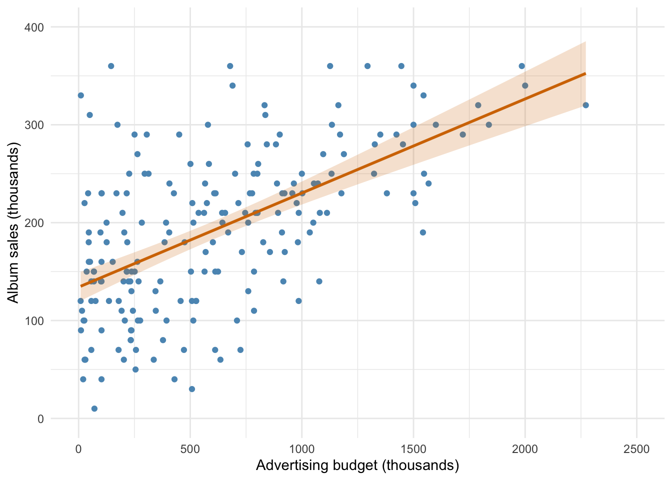
Scatterplot of album sales against advertising
ggplot2::ggplot(album_tib, aes(adverts, sales)) +
  geom_point(colour = "#5c97bf") +
  coord_cartesian(ylim = c(0, 400), xlim = c(0, 2500)) +
  scale_x_continuous(breaks = seq(0, 2500, 500)) +
  scale_y_continuous(breaks = seq(0, 400, 100)) +
  labs(x = "Advertising budget (thousands)", y = "Album sales (thousands)") +
  geom_smooth(method = "lm", colour = "#d47500", fill = "#d47500", alpha = 0.2) +
  theme_minimal()
Fit a model with one predictor
album_lm <- lm(sales ~ adverts, data = album_tib, na.action = na.exclude)
get text output for the model:
summary(album_lm)
##
## Call:
## lm(formula = sales ~ adverts, data = album_tib, na.action = na.exclude)
##
## Residuals:
##      Min       1Q   Median       3Q      Max
## -152.949  -43.796   -0.393   37.040  211.866
##
## Coefficients:
##              Estimate Std. Error t value Pr(>|t|)
## (Intercept) 1.341e+02  7.537e+00  17.799   <2e-16 ***
## adverts     9.612e-02  9.632e-03   9.979   <2e-16 ***
## ---
## Signif. codes:  0 '***' 0.001 '**' 0.01 '*' 0.05 '.' 0.1 ' ' 1
##
## Residual standard error: 65.99 on 198 degrees of freedom
## Multiple R-squared:  0.3346,	Adjusted R-squared:  0.3313
## F-statistic: 99.59 on 1 and 198 DF,  p-value: < 2.2e-16
Get the confidence intervals for the model parameters old-style:
confint(album_lm)
##                    2.5 %      97.5 %
## (Intercept) 119.27768082 149.0021948
## adverts       0.07712929   0.1151197
Or, better …. use broom() to get nicely tabulated fit statistics:
broom::glance(album_lm)
## # A tibble: 1 x 12
##   r.squared adj.r.squared sigma statistic  p.value    df logLik   AIC   BIC
##       <dbl>         <dbl> <dbl>     <dbl>    <dbl> <dbl>  <dbl> <dbl> <dbl>
## 1     0.335         0.331  66.0      99.6 2.94e-19     1 -1121. 2247. 2257.
## # … with 3 more variables: deviance <dbl>, df.residual <int>, nobs <int>
Finally, you can compute multiple R:
summary(album_lm)$r.squared %>%
  sqrt()
## [1] 0.5784877
Also use broom() to get nicely tabulated parameter estimates (including confidence intervals):
broom::tidy(album_lm, conf.int = TRUE)
## # A tibble: 2 x 7
##   term        estimate std.error statistic  p.value conf.low conf.high
##   <chr>          <dbl>     <dbl>     <dbl>    <dbl>    <dbl>     <dbl>
## 1 (Intercept) 134.       7.54        17.8  5.97e-43 119.       149.
## 2 adverts       0.0961   0.00963      9.98 2.94e-19   0.0771     0.115
Impress your friends by rounding values to 3 decimal places using mutate() and across()
broom::tidy(album_lm, conf.int = TRUE) %>%
  dplyr::mutate(
    dplyr::across(where(is.numeric), ~round(., 3))
  )
## # A tibble: 2 x 7
##   term        estimate std.error statistic p.value conf.low conf.high
##   <chr>          <dbl>     <dbl>     <dbl>   <dbl>    <dbl>     <dbl>
## 1 (Intercept)  134.         7.54     17.8        0  119.      149.
## 2 adverts        0.096      0.01      9.98       0    0.077     0.115
Or by using the pixiedust package:
broom::tidy(album_lm, conf.int = TRUE) %>%
  pixiedust::dust() %>%
  pixiedust::sprinkle(col = 2:7, round = 3)
| term | estimate | std.error | statistic | p.value | conf.low | conf.high |
|---|---|---|---|---|---|---|
| (Intercept) | 134.14 | 7.537 | 17.799 | 0 | 119.278 | 149.002 |
| adverts | 0.096 | 0.01 | 9.979 | 0 | 0.077 | 0.115 |
Fit a model with several predictor
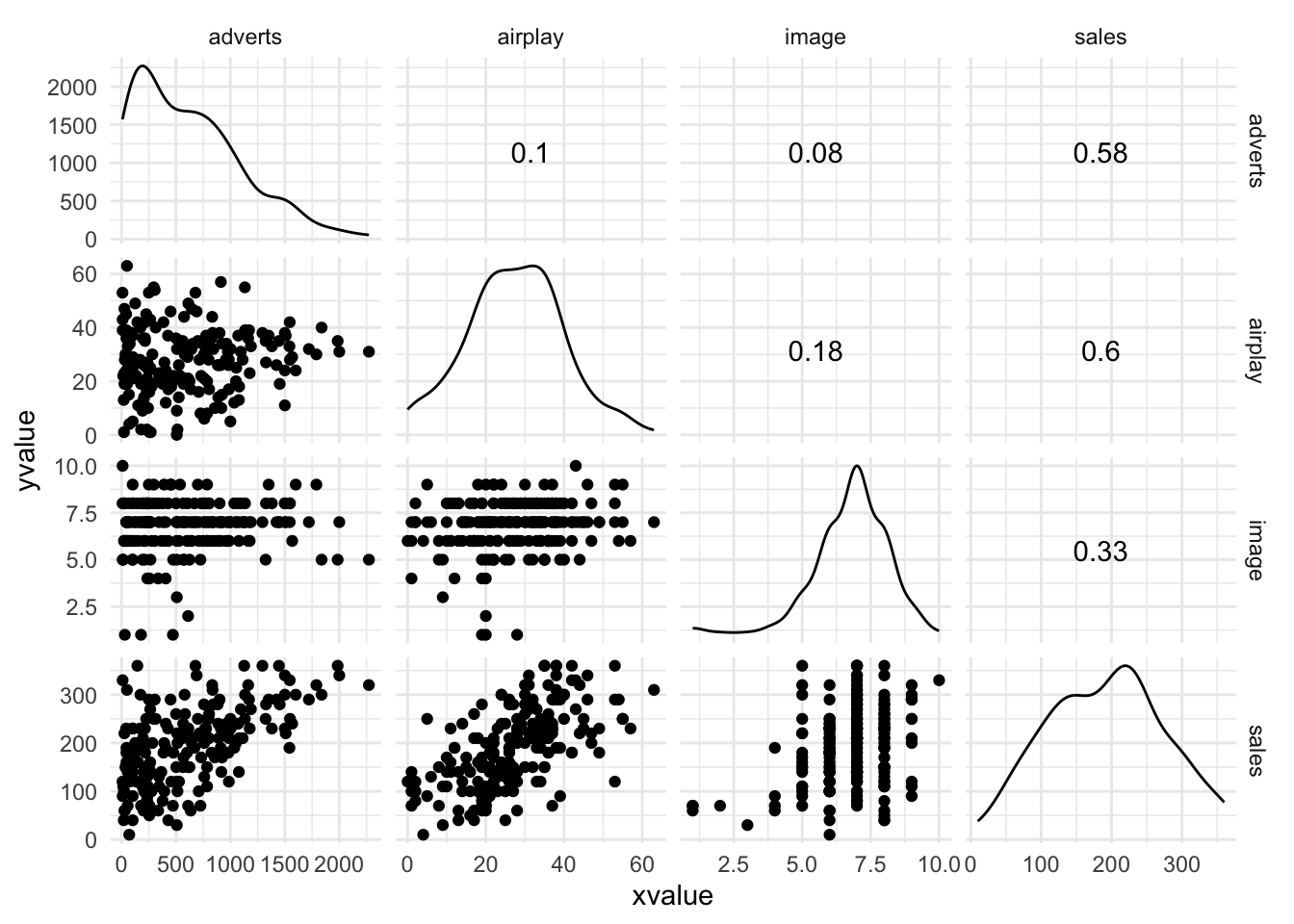
Bivariate correlations and scatterplots
Plot the data
GGally::ggscatmat(album_tib, columns = c("adverts", "airplay", "image", "sales")) +
  theme_minimal()
Build the model
album_full_lm <- lm(sales ~ adverts + airplay + image, data = album_tib, na.action = na.exclude)
Or, use the update function:
album_full_lm <- update(album_lm, .~. + airplay + image)
Fit statistics
broom::glance(album_full_lm)
## # A tibble: 1 x 12
##   r.squared adj.r.squared sigma statistic  p.value    df logLik   AIC   BIC
##       <dbl>         <dbl> <dbl>     <dbl>    <dbl> <dbl>  <dbl> <dbl> <dbl>
## 1     0.665         0.660  47.1      129. 2.88e-46     3 -1052. 2114. 2131.
## # … with 3 more variables: deviance <dbl>, df.residual <int>, nobs <int>
multiple R-square:
summary(album_full_lm)$r.squared %>%
  sqrt()
## [1] 0.8152715
Compare models
anova(album_lm, album_full_lm) %>%
  broom::tidy()
## # A tibble: 2 x 6
##   res.df     rss    df   sumsq statistic   p.value
##    <dbl>   <dbl> <dbl>   <dbl>     <dbl>     <dbl>
## 1    198 862264.    NA     NA       NA   NA
## 2    196 434575.     2 427690.      96.4  6.88e-30
Parameter estimates
As text:
summary(album_full_lm)
##
## Call:
## lm(formula = sales ~ adverts + airplay + image, data = album_tib,
##     na.action = na.exclude)
##
## Residuals:
##      Min       1Q   Median       3Q      Max
## -121.324  -28.336   -0.451   28.967  144.132
##
## Coefficients:
##               Estimate Std. Error t value Pr(>|t|)
## (Intercept) -26.612958  17.350001  -1.534    0.127
## adverts       0.084885   0.006923  12.261  < 2e-16 ***
## airplay       3.367425   0.277771  12.123  < 2e-16 ***
## image        11.086335   2.437849   4.548 9.49e-06 ***
## ---
## Signif. codes:  0 '***' 0.001 '**' 0.01 '*' 0.05 '.' 0.1 ' ' 1
##
## Residual standard error: 47.09 on 196 degrees of freedom
## Multiple R-squared:  0.6647,	Adjusted R-squared:  0.6595
## F-statistic: 129.5 on 3 and 196 DF,  p-value: < 2.2e-16
confint(album_full_lm)
##                    2.5 %      97.5 %
## (Intercept) -60.82960967  7.60369295
## adverts       0.07123166  0.09853799
## airplay       2.81962186  3.91522848
## image         6.27855218 15.89411823
As a nicely formatted table:
broom::tidy(album_full_lm, conf.int = TRUE)
## # A tibble: 4 x 7
##   term        estimate std.error statistic  p.value conf.low conf.high
##   <chr>          <dbl>     <dbl>     <dbl>    <dbl>    <dbl>     <dbl>
## 1 (Intercept) -26.6     17.4         -1.53 1.27e- 1 -60.8       7.60
## 2 adverts       0.0849   0.00692     12.3  5.05e-26   0.0712    0.0985
## 3 airplay       3.37     0.278       12.1  1.33e-25   2.82      3.92
## 4 image        11.1      2.44         4.55 9.49e- 6   6.28     15.9
Restrict the output to 3 decimal places
broom::tidy(album_full_lm, conf.int = TRUE) %>%
  dplyr::mutate(
    dplyr::across(where(is.numeric), ~round(., 3))
  )
## # A tibble: 4 x 7
##   term        estimate std.error statistic p.value conf.low conf.high
##   <chr>          <dbl>     <dbl>     <dbl>   <dbl>    <dbl>     <dbl>
## 1 (Intercept)  -26.6      17.4       -1.53   0.127  -60.8       7.60
## 2 adverts        0.085     0.007     12.3    0        0.071     0.099
## 3 airplay        3.37      0.278     12.1    0        2.82      3.92
## 4 image         11.1       2.44       4.55   0        6.28     15.9
Standardized betas
parameters::model_parameters(album_full_lm, standardize = "refit", digits = 3)
## Parameter   | Coefficient |    SE |        95% CI |          t |  df |      p
## -----------------------------------------------------------------------------
## (Intercept) |  -3.982e-17 | 0.041 | [-0.08, 0.08] | -9.650e-16 | 196 | > .999
## adverts     |       0.511 | 0.042 | [ 0.43, 0.59] |     12.261 | 196 | < .001
## airplay     |       0.512 | 0.042 | [ 0.43, 0.60] |     12.123 | 196 | < .001
## image       |       0.192 | 0.042 | [ 0.11, 0.27] |      4.548 | 196 | < .001
Influence measures
album_full_rsd <- album_full_lm %>%
  broom::augment() %>%
  tibble::rowid_to_column(var = "case_no")

album_full_rsd
## # A tibble: 200 x 11
##    case_no sales adverts airplay image .fitted  .resid .std.resid    .hat .sigma
##      <int> <dbl>   <dbl>   <dbl> <dbl>   <dbl>   <dbl>      <dbl>   <dbl>  <dbl>
##  1       1   330    10.3      43    10   230.  -100.        2.18  0.0472    46.6
##  2       2   120   986.       28     7   229.   109.       -2.32  0.00801   46.6
##  3       3   360  1446.       35     7   292.   -68.4       1.47  0.0207    46.9
##  4       4   270  1188.       33     7   263.    -7.02      0.150 0.0126    47.2
##  5       5   220   575.       44     5   226.     5.75     -0.124 0.0261    47.2
##  6       6   170   569.       19     5   141.   -28.9       0.618 0.0142    47.2
##  7       7    70   472.       20     1    91.9   21.9      -0.487 0.0910    47.2
##  8       8   210   537.       22     9   193.   -17.1       0.368 0.0209    47.2
##  9       9   200   514.       21     7   165.   -34.7       0.739 0.00691   47.1
## 10      10   300   174.       40     7   200.   -99.5       2.13  0.0154    46.7
## # … with 190 more rows, and 1 more variable: .cooksd <dbl>
album_full_inf <- influence.measures(album_full_lm)

album_full_inf <- album_full_inf$infmat %>%
  tibble::as_tibble() %>%
  tibble::rowid_to_column(var = "case_no")


album_full_inf
## # A tibble: 200 x 9
##    case_no   dfb.1_ dfb.advr dfb.arpl  dfb.imag   dffit cov.r    cook.d     hat
##      <int>    <dbl>    <dbl>    <dbl>     <dbl>   <dbl> <dbl>     <dbl>   <dbl>
##  1       1 -0.316   -0.242    0.158    0.353     0.489  0.971 0.0587    0.0472
##  2       2  0.0126  -0.126    0.00942 -0.0187   -0.211  0.920 0.0109    0.00801
##  3       3 -0.0381   0.175    0.0466  -0.00538   0.214  0.997 0.0114    0.0207
##  4       4 -0.00258  0.0122   0.00344  0.000129  0.0169 1.03  0.0000717 0.0126
##  5       5 -0.00858  0.00109 -0.0143   0.0136   -0.0202 1.05  0.000103  0.0261
##  6       6  0.0658   0.00224 -0.0208  -0.0512    0.0741 1.03  0.00138   0.0142
##  7       7 -0.145   -0.00100 -0.00509  0.148    -0.154  1.12  0.00594   0.0910
##  8       8 -0.0281  -0.00586 -0.0192   0.0452    0.0537 1.04  0.000723  0.0209
##  9       9  0.0112  -0.00896 -0.0290   0.0145    0.0615 1.02  0.000949  0.00691
## 10      10 -0.0126  -0.156    0.168    0.00672   0.269  0.944 0.0178    0.0154
## # … with 190 more rows
If you want to keep all of your diagnostic stats in one object:
album_full_rsd <- album_full_rsd %>%
  dplyr::left_join(., album_full_inf, by = "case_no") %>%
  dplyr::select(-c(cook.d, hat))
Variance inflation factor
car::vif(album_full_lm)
##  adverts  airplay    image
## 1.014593 1.042504 1.038455
1/car::vif(album_full_lm)
##   adverts   airplay     image
## 0.9856172 0.9592287 0.9629695
car::vif(album_full_lm) %>%
  mean()
## [1] 1.03185
Casewise diagnostics
get_cum_percent <- function(var,  cut_off = 1.96){
  ecdf_var <- abs(var) %>% ecdf()
  100*(1 - ecdf_var(cut_off))
}


album_full_rsd %>%
  dplyr::summarize(
    `z >= 1.96` = get_cum_percent(.std.resid),
    `z >= 2.58` = get_cum_percent(.std.resid, cut_off = 2.58),
    `z >= 3.29` = get_cum_percent(.std.resid, cut_off = 3.29)
  )
## # A tibble: 1 x 3
##   `z >= 1.96` `z >= 2.58` `z >= 3.29`
##         <dbl>       <dbl>       <dbl>
## 1        6.50          1.           0
album_full_rsd %>%
  dplyr::filter(abs(.std.resid) >= 1.96) %>%
  dplyr::select(case_no, .std.resid, .resid) %>%
  dplyr::arrange(.std.resid)
## # A tibble: 13 x 3
##    case_no .std.resid .resid
##      <int>      <dbl>  <dbl>
##  1     164      -2.63  121.
##  2      47      -2.46  115.
##  3      55      -2.46  114.
##  4      68      -2.36  110.
##  5       2      -2.32  109.
##  6     200      -2.09   97.2
##  7     167      -2.00   93.6
##  8     100       2.10  -97.3
##  9      52       2.10  -97.4
## 10      61       2.10  -98.8
## 11      10       2.13  -99.5
## 12       1       2.18 -100.
## 13     169       3.09 -144.
album_full_inf %>%
  dplyr::arrange(desc(cook.d)) %>%
  dplyr::mutate(
    dplyr::across(where(is.numeric), ~round(., 3))
  )
## # A tibble: 200 x 9
##    case_no dfb.1_ dfb.advr dfb.arpl dfb.imag  dffit cov.r cook.d   hat
##      <dbl>  <dbl>    <dbl>    <dbl>    <dbl>  <dbl> <dbl>  <dbl> <dbl>
##  1     164  0.18     0.290   -0.401   -0.117 -0.54  0.92   0.071 0.039
##  2       1 -0.316   -0.242    0.158    0.353  0.489 0.971  0.059 0.047
##  3     169 -0.168   -0.258    0.257    0.17   0.461 0.853  0.051 0.021
##  4      55  0.174   -0.326   -0.023   -0.124 -0.407 0.925  0.04  0.026
##  5      52  0.353   -0.029   -0.137   -0.27   0.367 0.96   0.033 0.029
##  6     100  0.061    0.145   -0.3      0.068  0.357 0.959  0.031 0.028
##  7     119  0.004   -0.054   -0.312    0.129 -0.353 1.00   0.031 0.04
##  8      99  0.088   -0.111   -0.279    0.039 -0.337 0.99   0.028 0.034
##  9     200  0.166   -0.046    0.142   -0.259 -0.32  0.954  0.025 0.023
## 10      47  0.066    0.196    0.048   -0.179 -0.315 0.915  0.024 0.016
## # … with 190 more rows
Show case with any df beta with an absolute value greater than 1.
album_full_inf %>%
  dplyr::filter_at(
    vars(starts_with("dfb")),
    any_vars(abs(.) > 1)
  ) %>%
  dplyr::select(case_no, starts_with("dfb")) %>%
  dplyr::mutate(
    dplyr::across(where(is.numeric), ~round(., 3))
  )
## # A tibble: 0 x 5
## # … with 5 variables: case_no <dbl>, dfb.1_ <dbl>, dfb.advr <dbl>,
## #   dfb.arpl <dbl>, dfb.imag <dbl>
Show cases with problematic leverage or CVR:
leverage_thresh <- 3*mean(album_full_inf$hat, na.rm = TRUE)

album_full_inf %>%
  dplyr::filter(
    hat > leverage_thresh | !between(cov.r, 1 - leverage_thresh, 1 + leverage_thresh)
    ) %>%
  dplyr::select(case_no, cov.r, hat, cook.d) %>%
  dplyr::mutate(
    dplyr::across(where(is.numeric), ~round(., 3))
  )
## # A tibble: 21 x 4
##    case_no cov.r   hat cook.d
##      <dbl> <dbl> <dbl>  <dbl>
##  1       2 0.92  0.008  0.011
##  2       7 1.12  0.091  0.006
##  3      12 1.07  0.064  0.017
##  4      23 1.07  0.045  0
##  5      42 1.06  0.058  0.013
##  6      43 1.07  0.046  0.001
##  7      47 0.915 0.016  0.024
##  8      55 0.925 0.026  0.04
##  9      61 0.937 0.005  0.006
## 10      68 0.924 0.016  0.022
## # … with 11 more rows
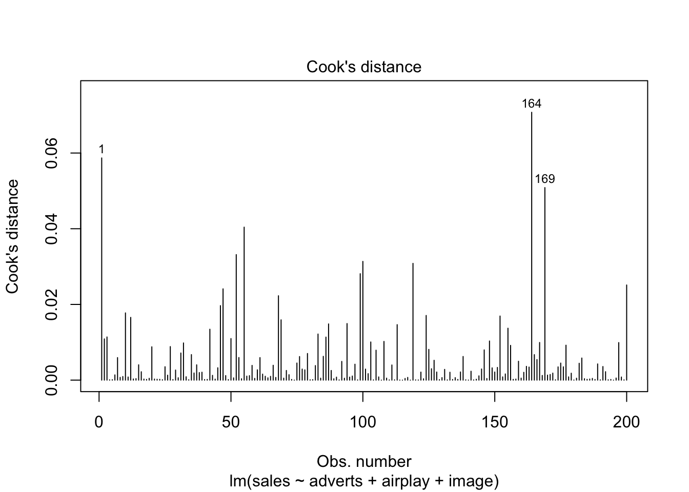
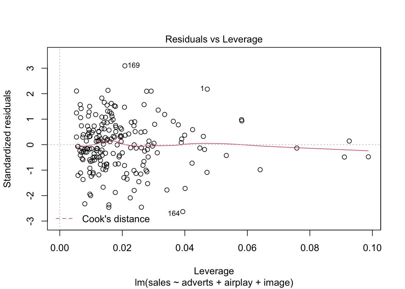
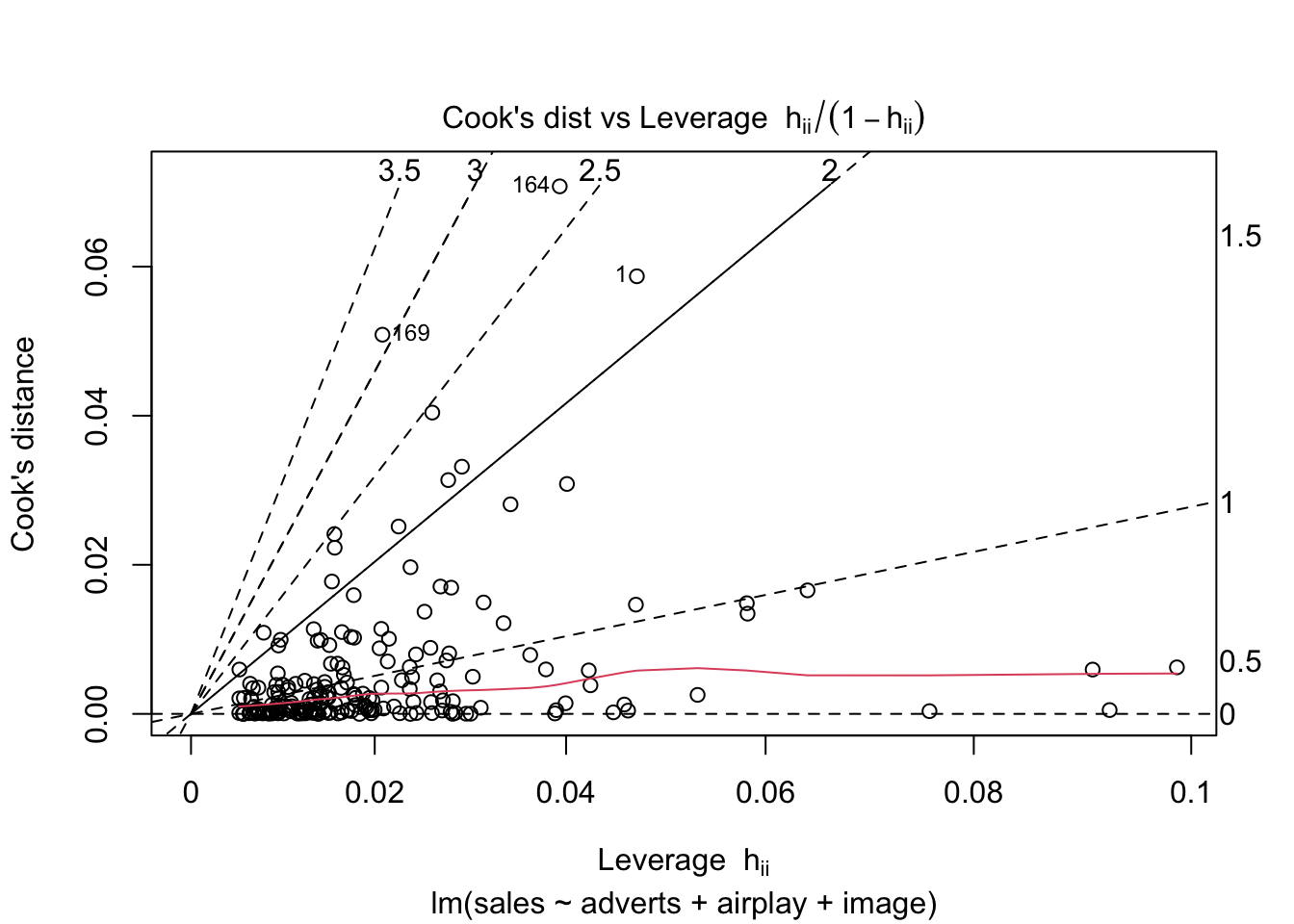
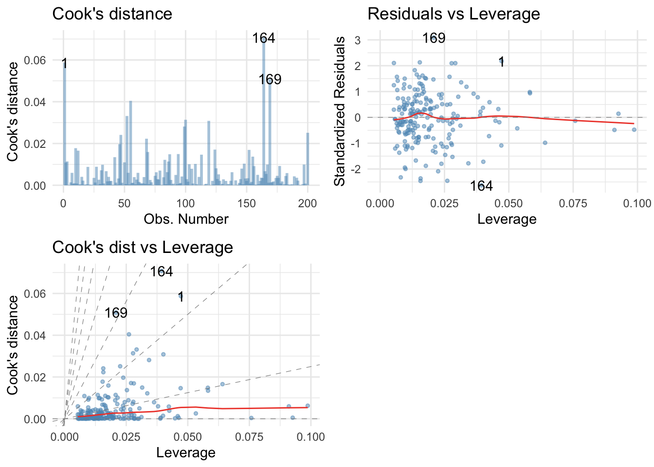
Diagnostic plots
Standard influence plots
plot(album_full_lm, which = 4:6)
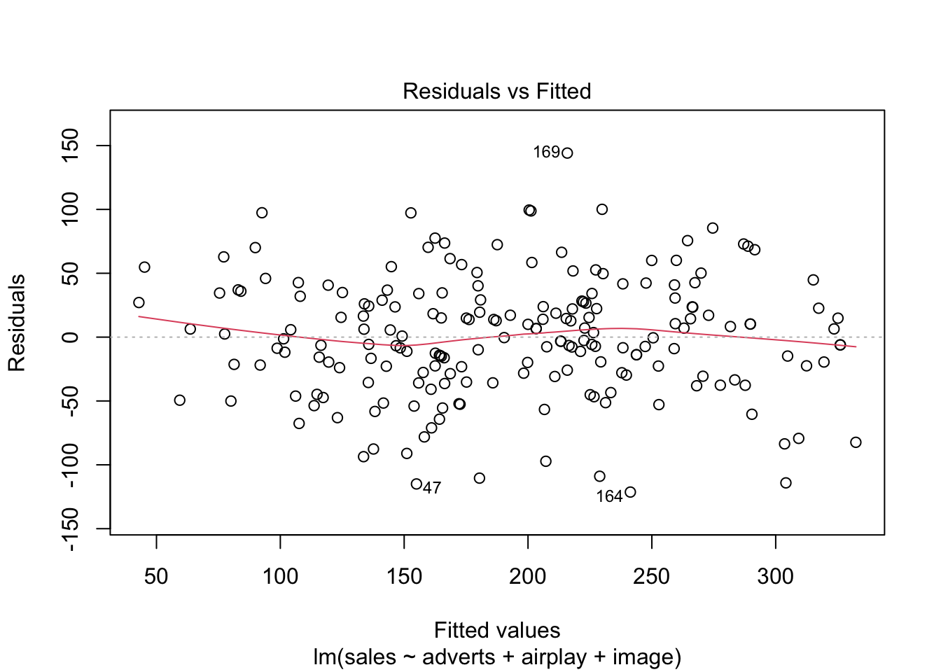
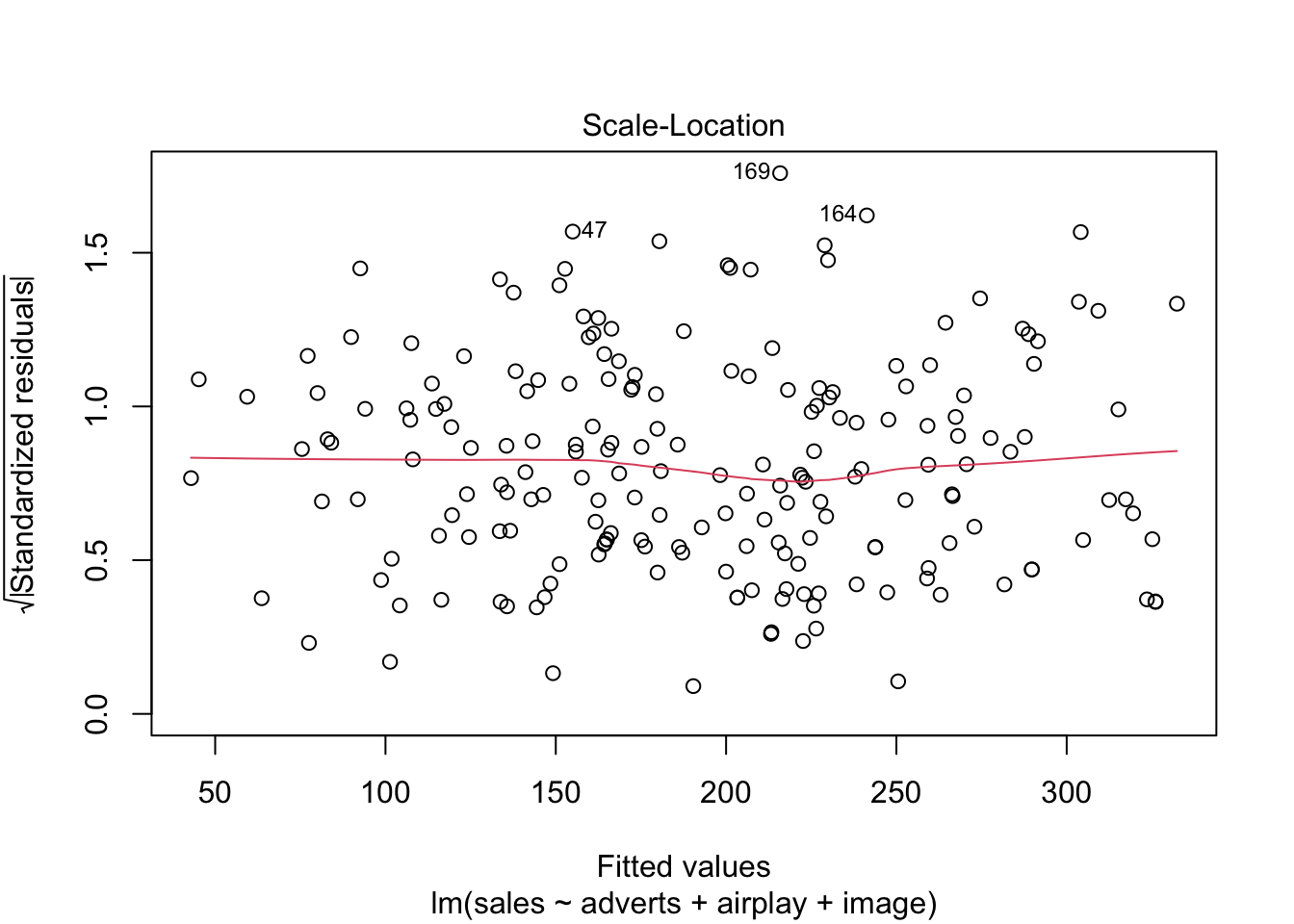
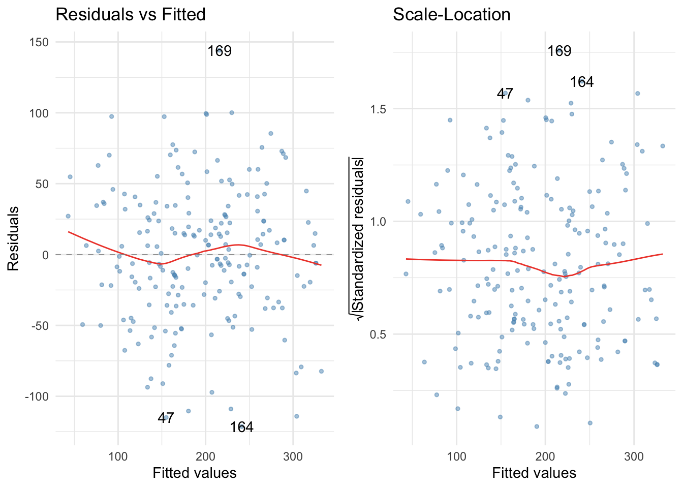
Residual plot:
plot(album_full_lm, which = c(1, 3))
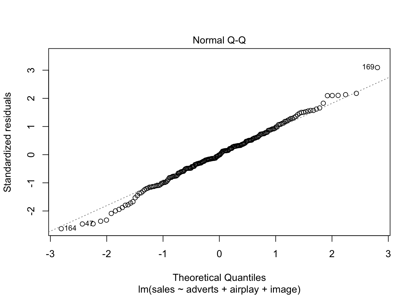
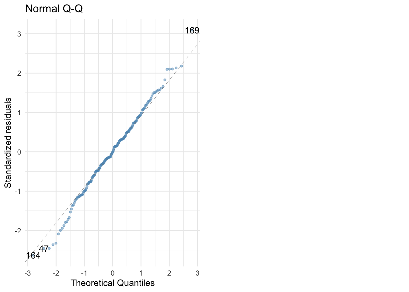
Q-Q plot:
plot(album_full_lm, which = 2)
Prettier diagnostic plots
The ggfortify package allows us to produce prettier versions of the diagnostic plots. For example:
influence plots
library(ggfortify)
ggplot2::autoplot(album_full_lm, which = 4:6,
                  colour = "#5c97bf",
                  smooth.colour = "#ef4836",
                  alpha = 0.5,
                  size = 1) +
  theme_minimal()
Residual plot:
ggplot2::autoplot(album_full_lm, which = c(1, 3),
                  colour = "#5c97bf",
                  smooth.colour = "#ef4836",
                  alpha = 0.5,
                  size = 1) +
  theme_minimal()
Q-Q plot:
ggplot2::autoplot(album_full_lm, which = 2,
                  colour = "#5c97bf",
                  smooth.colour = "#ef4836",
                  alpha = 0.5,
                  size = 1) +
  theme_minimal()
Robust linear model
Robust estimates:
album_full_rob <- robust::lmRob(sales ~ adverts + airplay + image, data = album_tib, na.action = na.exclude)
summary(album_full_rob)
##
## Call:
## robust::lmRob(formula = sales ~ adverts + airplay + image, data = album_tib,
##     na.action = na.exclude)
##
## Residuals:
##     Min      1Q  Median      3Q     Max
## -124.62  -30.47   -1.76   28.89  141.35
##
## Coefficients:
##               Estimate Std. Error t value Pr(>|t|)
## (Intercept) -31.523201  21.098348  -1.494 0.136756
## adverts       0.085295   0.008501  10.033  < 2e-16 ***
## airplay       3.418749   0.339017  10.084  < 2e-16 ***
## image        11.771441   2.973559   3.959 0.000105 ***
## ---
## Signif. codes:  0 '***' 0.001 '**' 0.01 '*' 0.05 '.' 0.1 ' ' 1
##
## Residual standard error: 44.61 on 196 degrees of freedom
## Multiple R-Squared: 0.5785
##
## Test for Bias:
##             statistic p-value
## M-estimate      2.299  0.6809
## LS-estimate     7.659  0.1049
Robust standard errors and confidence intervals:
parameters::model_parameters(
  album_full_lm,
  robust = TRUE,
  vcov.type = "HC4",
  digits = 3
  )
## Parameter   | Coefficient |     SE |          95% CI |      t |  df |      p
## ----------------------------------------------------------------------------
## (Intercept) |     -26.613 | 16.170 | [-58.50,  5.28] | -1.646 | 196 | 0.101
## adverts     |       0.085 |  0.007 | [  0.07,  0.10] | 12.246 | 196 | < .001
## airplay     |       3.367 |  0.315 | [  2.75,  3.99] | 10.687 | 196 | < .001
## image       |      11.086 |  2.247 | [  6.65, 15.52] |  4.933 | 196 | < .001
Bootstrap
parameters::model_parameters(
  album_full_lm,
  bootstrap = TRUE,
  digits = 3
  )
## Parameter   | Coefficient |          95% CI |      p
## ----------------------------------------------------
## (Intercept) |     -26.928 | [-55.65,  7.06] | 0.116
## adverts     |       0.085 | [  0.07,  0.10] | < .001
## airplay     |       3.366 | [  2.74,  4.02] | < .001
## image       |      11.059 | [  6.36, 15.40] | < .001
Bayes factors
album_bf <- album_tib %>%
  BayesFactor::regressionBF(sales ~ adverts + airplay + image, rscaleCont = "medium", data = .)

album_bf
## Bayes factor analysis
## --------------
## [1] adverts                   : 1.320123e+16 ±0%
## [2] airplay                   : 4.723817e+17 ±0.01%
## [3] image                     : 6039.289     ±0%
## [4] adverts + airplay         : 5.65038e+39  ±0%
## [5] adverts + image           : 2.65494e+20  ±0%
## [6] airplay + image           : 1.034464e+20 ±0%
## [7] adverts + airplay + image : 7.746101e+42 ±0%
##
## Against denominator:
##   Intercept only
## ---
## Bayes factor type: BFlinearModel, JZS
Bayesian parameter estimates
album_full_bf <- album_tib %>%
  BayesFactor::lmBF(sales ~ adverts + airplay + image, rscaleCont = "medium", data = .)

album_full_post <- BayesFactor::posterior(album_full_bf, iterations = 10000)
summary(album_full_post)
##
## Iterations = 1:10000
## Thinning interval = 1
## Number of chains = 1
## Sample size per chain = 10000
##
## 1. Empirical mean and standard deviation for each variable,
##    plus standard error of the mean:
##
##              Mean        SD  Naive SE Time-series SE
## mu      1.932e+02 3.309e+00 3.309e-02      3.309e-02
## adverts 8.406e-02 7.038e-03 7.038e-05      7.038e-05
## airplay 3.333e+00 2.804e-01 2.804e-03      2.804e-03
## image   1.096e+01 2.475e+00 2.475e-02      2.475e-02
## sig2    2.253e+03 2.321e+02 2.321e+00      2.313e+00
## g       9.859e-01 1.553e+00 1.553e-02      1.553e-02
##
## 2. Quantiles for each variable:
##
##              2.5%       25%       50%       75%     97.5%
## mu      1.868e+02 1.909e+02 1.932e+02 1.954e+02 1.998e+02
## adverts 7.004e-02 7.932e-02 8.412e-02 8.882e-02 9.798e-02
## airplay 2.780e+00 3.145e+00 3.336e+00 3.522e+00 3.872e+00
## image   6.056e+00 9.269e+00 1.097e+01 1.266e+01 1.571e+01
## sig2    1.841e+03 2.092e+03 2.239e+03 2.395e+03 2.750e+03
## g       1.770e-01 3.708e-01 6.017e-01 1.047e+00 4.203e+00