R code Chapter 7

This document contains abridged sections from Discovering Statistics Using R and RStudio by Andy Field so there are some copyright considerations. You can use this material for teaching and non-profit activities but please do not meddle with it or claim it as your own work. See the full license terms at the bottom of the page.
Load the data
Remember to install the package for the book with library(discovr). After which you can load data into a tibble by executing:
name_of_tib <- discovr::name_of_data
For example, execute these lines to create the tibbles referred to in the chapter:
cats_tib <- discovr::roaming_cats
exam_tib <- discovr::exam_anxiety
liar_tib <- discovr::biggest_liar
If you want to read the file from the CSV and you have set up your project folder as I suggest in Chapter 1, then the general format of the code you would use is:
tibble_name <- here::here("../data/name_of_file.csv") %>%
  readr::read_csv() %>%
  dplyr::mutate(
    ...
    code to convert character variables to factors
    ...
  )
In which you’d replace tibble_name with the name you want to assign to the tibble and change name_of_file.csv to the name of the file that you’re trying to load. You can use mutate to convert categorical variables to factors. For example, for the exam_anxiety data you would load it by executing:
exam_tib <- here::here("data/exam_anxiety.csv") %>%
  readr::read_csv() %>%
  dplyr::mutate(
    sex = forcats::as_factor(sex)
  )
Bivariate correlations
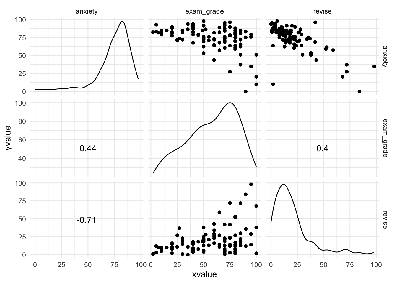
Plot the data
GGally::ggscatmat(exam_tib, columns = c("exam_grade", "revise", "anxiety")) +
  theme_minimal()
Pearson’s r
A single correlation:
exam_tib %>%
  dplyr::select(exam_grade, revise) %>%
  correlation::correlation()
## Parameter1 | Parameter2 |    r |       95% CI |    t |  df |      p |  Method | n_Obs
## -------------------------------------------------------------------------------------
## exam_grade |     revise | 0.40 | [0.22, 0.55] | 4.34 | 101 | < .001 | Pearson |   103
Let’s scale this up to include exam anxiety:
exam_cor <- exam_tib %>%
  dplyr::select(exam_grade, revise, anxiety) %>%
  correlation::correlation()

exam_cor
## Parameter1 | Parameter2 |     r |         95% CI |      t |  df |      p |  Method | n_Obs
## ------------------------------------------------------------------------------------------
## exam_grade |     revise |  0.40 | [ 0.22,  0.55] |   4.34 | 101 | < .001 | Pearson |   103
## exam_grade |    anxiety | -0.44 | [-0.58, -0.27] |  -4.94 | 101 | < .001 | Pearson |   103
## revise     |    anxiety | -0.71 | [-0.79, -0.60] | -10.11 | 101 | < .001 | Pearson |   103
Change the number of decimal places
exam_tib %>%
  dplyr::select(exam_grade, revise, anxiety) %>%
  correlation::correlation(digits = 3, ci_digits = 3)
## Parameter1 | Parameter2 |      r |           95% CI |       t |  df |      p |  Method | n_Obs
## ----------------------------------------------------------------------------------------------
## exam_grade |     revise |  0.397 | [ 0.220,  0.548] |   4.343 | 101 | < .001 | Pearson |   103
## exam_grade |    anxiety | -0.441 | [-0.585, -0.271] |  -4.938 | 101 | < .001 | Pearson |   103
## revise     |    anxiety | -0.709 | [-0.794, -0.598] | -10.111 | 101 | < .001 | Pearson |   103
Matrix format
exam_tib %>%
  dplyr::select(exam_grade, revise, anxiety) %>%
  correlation::correlation() %>%
  summary()
## Parameter  |  anxiety |  revise
## -------------------------------
## exam_grade | -0.44*** | 0.40***
## revise     | -0.71*** |
Coefficient of determination
exam_cor <- exam_tib %>%
  dplyr::select(exam_grade, revise, anxiety) %>%
  correlation::correlation()

(exam_cor$r)^2
## [1] 0.1573873 0.1944752 0.5030345
Robust correlations
exam_tib %>%
  dplyr::select(exam_grade, revise, anxiety) %>%
  WRS2::winall()
## Call:
## WRS2::winall(x = .)
##
## Robust correlation matrix:
##            exam_grade  revise anxiety
## exam_grade     1.0000  0.3085 -0.3913
## revise         0.3085  1.0000 -0.6015
## anxiety       -0.3913 -0.6015  1.0000
##
## p-values:
##            exam_grade  revise anxiety
## exam_grade         NA 0.00183   7e-05
## revise        0.00183      NA   0e+00
## anxiety       0.00007 0.00000      NA
exam_tib %>%
  dplyr::select(exam_grade, revise, anxiety) %>%
  correlation::correlation(., method = "percentage")
## Parameter1 | Parameter2 |     r |         95% CI |     t |  df |      p |          Method | n_Obs
## -------------------------------------------------------------------------------------------------
## exam_grade |     revise |  0.34 | [ 0.15,  0.50] |  3.60 | 101 | < .001 | Percentage Bend |   103
## exam_grade |    anxiety | -0.40 | [-0.55, -0.23] | -4.41 | 101 | < .001 | Percentage Bend |   103
## revise     |    anxiety | -0.61 | [-0.72, -0.47] | -7.66 | 101 | < .001 | Percentage Bend |   103
Spearman’s rho
Load the Biggest Liar data from the CSV file (assuming you’ve set up a project as described in chapter 1)
liar_tib <- readr::read_csv("../data/biggest_liar.csv") %>%
  dplyr::mutate(
    novice = forcats::as_factor(novice)
  )
liar_tib %>%
  dplyr::select(position, creativity) %>%
  correlation::correlation(method = "spearman")
## Parameter1 | Parameter2 |   rho |         95% CI |        S |     p |   Method | n_Obs
## --------------------------------------------------------------------------------------
## position   | creativity | -0.38 | [-0.56, -0.15] | 72123.51 | 0.002 | Spearman |    68
Kendall’s tau
liar_tib %>%
  dplyr::select(position, creativity) %>%
  correlation::correlation(method = "kendall")
## Parameter1 | Parameter2 |         95% CI |   tau |     z |     p |  Method | n_Obs
## ----------------------------------------------------------------------------------
## position   | creativity | [-0.50, -0.07] | -0.30 | -3.24 | 0.001 | Kendall |    68
Bootstrapped confidence intervals
A quick aside, let’s look at the code for writing a function to print the mean:
print_mean <- function(variable){
	mean <- sum(variable)/nrow(variable)
       cat("Mean = ", mean)
}

exam_tib %>%
  dplyr::select(exam_grade) %>%
  print_mean()
## Mean = 56.57282
Or a sillier version:
print_mean <- function(harry_the_hungy_hippo){
	mean <- sum(harry_the_hungy_hippo)/ nrow(harry_the_hungy_hippo)
       cat("Harry the hungry hippo say that the mean = ", mean)
}

exam_tib %>%
  dplyr::select(exam_grade) %>%
  print_mean()
## Harry the hungry hippo say that the mean = 56.57282
Here’s a function to bootstrap Pearson’s r:
boot_r <- function(data, i){
  cor(data[i, "exam_grade"], data[i, "revise"])
}

grade_revise_bs <- boot::boot(exam_tib, boot_r, R = 2000)

grade_revise_bs
##
## ORDINARY NONPARAMETRIC BOOTSTRAP
##
##
## Call:
## boot::boot(data = exam_tib, statistic = boot_r, R = 2000)
##
##
## Bootstrap Statistics :
##      original       bias    std. error
## t1* 0.3967207 -0.001476077  0.06983568
boot::boot.ci(grade_revise_bs)
## BOOTSTRAP CONFIDENCE INTERVAL CALCULATIONS
## Based on 2000 bootstrap replicates
##
## CALL :
## boot::boot.ci(boot.out = grade_revise_bs)
##
## Intervals :
## Level      Normal              Basic
## 95%   ( 0.2613,  0.5351 )   ( 0.2673,  0.5424 )
##
## Level     Percentile            BCa
## 95%   ( 0.2510,  0.5261 )   ( 0.2530,  0.5263 )
## Calculations and Intervals on Original Scale
A general bootstrap function
boot_r <- function(data, var1, var2, i){
  cor(data[i, var1], data[i, var2])
}

grade_revise_bs <- boot::boot(exam_tib, boot_r, var1 = "exam_grade", var2 = "revise", R = 2000)
grade_revise_bs
##
## ORDINARY NONPARAMETRIC BOOTSTRAP
##
##
## Call:
## boot::boot(data = exam_tib, statistic = boot_r, R = 2000, var1 = "exam_grade",
##     var2 = "revise")
##
##
## Bootstrap Statistics :
##      original       bias    std. error
## t1* 0.3967207 -0.001593843  0.06788372
boot::boot.ci(grade_revise_bs)
## BOOTSTRAP CONFIDENCE INTERVAL CALCULATIONS
## Based on 2000 bootstrap replicates
##
## CALL :
## boot::boot.ci(boot.out = grade_revise_bs)
##
## Intervals :
## Level      Normal              Basic
## 95%   ( 0.2653,  0.5314 )   ( 0.2732,  0.5405 )
##
## Level     Percentile            BCa
## 95%   ( 0.2529,  0.5202 )   ( 0.2518,  0.5198 )
## Calculations and Intervals on Original Scale
grade_anx_bs <- boot::boot(exam_tib, boot_r, var1 = "exam_grade", var2 = "anxiety", R = 2000)
grade_anx_bs
##
## ORDINARY NONPARAMETRIC BOOTSTRAP
##
##
## Call:
## boot::boot(data = exam_tib, statistic = boot_r, R = 2000, var1 = "exam_grade",
##     var2 = "anxiety")
##
##
## Bootstrap Statistics :
##       original      bias    std. error
## t1* -0.4409934 0.002270827   0.0644994
boot::boot.ci(grade_anx_bs)
## BOOTSTRAP CONFIDENCE INTERVAL CALCULATIONS
## Based on 2000 bootstrap replicates
##
## CALL :
## boot::boot.ci(boot.out = grade_anx_bs)
##
## Intervals :
## Level      Normal              Basic
## 95%   (-0.5697, -0.3168 )   (-0.5767, -0.3235 )
##
## Level     Percentile            BCa
## 95%   (-0.5585, -0.3053 )   (-0.5609, -0.3088 )
## Calculations and Intervals on Original Scale
revise_anx_bs <- boot::boot(exam_tib, boot_r, var1 = "revise", var2 = "anxiety", R = 2000)
revise_anx_bs
##
## ORDINARY NONPARAMETRIC BOOTSTRAP
##
##
## Call:
## boot::boot(data = exam_tib, statistic = boot_r, R = 2000, var1 = "revise",
##     var2 = "anxiety")
##
##
## Bootstrap Statistics :
##       original      bias    std. error
## t1* -0.7092493 0.001022998    0.108373
boot::boot.ci(revise_anx_bs)
## BOOTSTRAP CONFIDENCE INTERVAL CALCULATIONS
## Based on 2000 bootstrap replicates
##
## CALL :
## boot::boot.ci(boot.out = revise_anx_bs)
##
## Intervals :
## Level      Normal              Basic
## 95%   (-0.9227, -0.4979 )   (-0.9525, -0.5483 )
##
## Level     Percentile            BCa
## 95%   (-0.8702, -0.4660 )   (-0.8530, -0.3760 )
## Calculations and Intervals on Original Scale
Bootrapping Spearman’s rho and Kendall’s tau
boot_r <- function(data, var1, var2, method = "pearson", i){
  cor(data[i, var1], data[i, var2], method = method)
}

liar_bs <- boot::boot(liar_tib, boot_r, var1 = "position", var2 = "creativity", method = "spearman", R = 2000)
boot::boot.ci(liar_bs)
## BOOTSTRAP CONFIDENCE INTERVAL CALCULATIONS
## Based on 2000 bootstrap replicates
##
## CALL :
## boot::boot.ci(boot.out = liar_bs)
##
## Intervals :
## Level      Normal              Basic
## 95%   (-0.6204, -0.1376 )   (-0.6294, -0.1555 )
##
## Level     Percentile            BCa
## 95%   (-0.5976, -0.1238 )   (-0.5818, -0.1042 )
## Calculations and Intervals on Original Scale
Point-biserial correlation
If you need to read the data in from the csv file:
cats_tib <- readr::read_csv("../data/roaming_cats.csv") %>%
  dplyr::mutate(
    sex = forcats::as_factor(sex)
  )
cats_tib <- cats_tib %>%
  dplyr::mutate(
    sex_bin = ifelse(sex == "Male", 0, 1),
    sex_bin_recode = ifelse(sex == "Male", 1, 0)
  )
cats_tib %>%
  dplyr::select(time, sex_bin) %>%
  correlation::correlation()
## Parameter1 | Parameter2 |     r |         95% CI |     t | df |     p |  Method | n_Obs
## ---------------------------------------------------------------------------------------
## time       |    sex_bin | -0.38 | [-0.58, -0.14] | -3.11 | 58 | 0.003 | Pearson |    60
coefficient of determination
r_cat <- cats_tib %>%
  dplyr::select(time, sex_bin) %>%
  correlation::correlation()

(r_cat$r)^2
## [1] 0.1432276
cats_tib %>%
  dplyr::select(time, sex_bin_recode) %>%
  correlation::correlation()
## Parameter1 |     Parameter2 |    r |       95% CI |    t | df |     p |  Method | n_Obs
## ---------------------------------------------------------------------------------------
## time       | sex_bin_recode | 0.38 | [0.14, 0.58] | 3.11 | 58 | 0.003 | Pearson |    60
cats_tib %>%
  dplyr::select(time, sex_bin) %>%
  correlation::correlation(method = "biserial")
## Parameter1 | Parameter2 |   rho |         95% CI |     t | df |      p |   Method | n_Obs
## -----------------------------------------------------------------------------------------
## time       |    sex_bin | -0.47 | [-0.65, -0.25] | -4.03 | 58 | < .001 | Biserial |    60
Partial correlations
exam_tib %>%
  dplyr::select(exam_grade, revise, anxiety) %>%
  correlation::correlation(., partial = TRUE)
## Parameter1 | Parameter2 |     r |         95% CI |     t |  df |      p |  Method | n_Obs
## -----------------------------------------------------------------------------------------
## exam_grade |     revise |  0.13 | [-0.06,  0.32] |  1.35 | 101 | 0.182  | Pearson |   103
## exam_grade |    anxiety | -0.25 | [-0.42, -0.06] | -2.56 | 101 | 0.024  | Pearson |   103
## revise     |    anxiety | -0.65 | [-0.75, -0.52] | -8.56 | 101 | < .001 | Pearson |   103
Comparing rs
The correlation between exam grade and anxiety for self-identifying males:
exam_tib %>%
  dplyr::filter(sex == "Male") %>%
  dplyr::select(exam_grade, anxiety) %>%
  correlation::correlation()
## Parameter1 | Parameter2 |     r |         95% CI |     t | df |      p |  Method | n_Obs
## ----------------------------------------------------------------------------------------
## exam_grade |    anxiety | -0.51 | [-0.68, -0.27] | -4.14 | 50 | < .001 | Pearson |    52
The correlation between exam grade and anxiety for self-identifying females:
exam_tib %>%
  dplyr::filter(sex == "Female") %>%
  dplyr::select(exam_grade, anxiety) %>%
  correlation::correlation()
## Parameter1 | Parameter2 |     r |         95% CI |     t | df |     p |  Method | n_Obs
## ---------------------------------------------------------------------------------------
## exam_grade |    anxiety | -0.38 | [-0.59, -0.12] | -2.89 | 49 | 0.006 | Pearson |    51
exam_male <- exam_tib %>%
  dplyr::filter(sex == "Male")

exam_female <- exam_tib %>%
  dplyr::filter(sex == "Female")

WRS2::twopcor(x1 = exam_male$exam_grade, y1 = exam_male$anxiety, x2 = exam_female$exam_grade, y2 = exam_female$anxiety)
## Call:
## WRS2::twopcor(x1 = exam_male$exam_grade, y1 = exam_male$anxiety,
##     x2 = exam_female$exam_grade, y2 = exam_female$anxiety)
##
## First correlation coefficient: -0.5057
## Second correlation coefficient: -0.3814
## Confidence interval (difference): -0.4574 0.1315