R code Chapter 6

This document contains abridged sections from Discovering Statistics Using R and RStudio by Andy Field so there are some copyright considerations. You can use this material for teaching and non-profit activities but please do not meddle with it or claim it as your own work. See the full license terms at the bottom of the page.
Load general packages
Remember to load the tidyverse:
library(tidyverse)
Load the data
Remember to install the package for the book with library(discovr). After which you can load data into a tibble by executing:
name_of_tib <- discovr::name_of_data
For example, execute these lines to create the tibbles referred to in the chapter:
download_tib <- discovr::download
If you want to read the file from the CSV and you have set up your project folder as I suggest in Chapter 1, then the general format of the code you would use is:
tibble_name <- here::here("../data/name_of_file.csv") %>%
  readr::read_csv() %>%
  dplyr::mutate(
    ...
    code to convert character variables to factors
    ...
  )
In which you’d replace tibble_name with the name you want to assign to the tibble and change name_of_file.csv to the name of the file that you’re trying to load. You can use mutate to convert categorical variables to factors. For example, for the download data you would load it by executing:
library(here)

download_tib <- here::here("data/download_festival.csv") %>%
  readr::read_csv() %>%
  dplyr::mutate(
    ticket_no = as.character(ticket_no),
    gender = forcats::as_factor(gender) %>% forcats::fct_relevel(., "Male", "Female", "Non-binary")
  )
Self-test
The original data: 1, 3, 4, 3, 2. The mean and sum of squares are:
friends <- c(1, 3, 4, 3, 2)
mean_old <- mean(friends)
ss_old <- (friends-mean_old)^2 %>% sum(.)

print(paste0("Original mean: ", mean_old))
## [1] "Original mean: 2.6"
print(paste0("Original SS: ", ss_old))
## [1] "Original SS: 5.2"
The data with the 4 replaced with a 10: 1, 3, 10, 3, and 2. The mean and sum of squares are:
friends_out <- c(1, 3, 10, 3, 2)
mean_out <- mean(friends_out)
ss_out <- (friends_out-mean_out)^2 %>% sum(.)

print(paste0("Mean with outlier: ", mean_out))
## [1] "Mean with outlier: 3.8"
print(paste0("SS with outlier: ", ss_out))
## [1] "SS with outlier: 50.8"
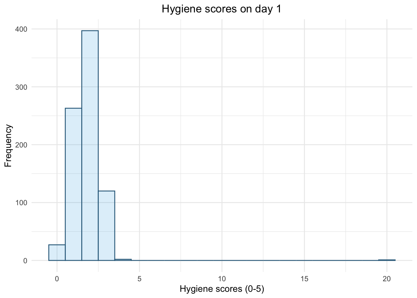
plot histogram
ggplot2::ggplot(download_tib, aes(day_1)) +
  geom_histogram(binwidth = 1, fill = "#56B4E9", colour = "#336c8b", alpha = 0.2) +
  labs(y = "Frequency", x = "Hygiene scores (0-5)", title = "Hygiene scores on day 1") +
  theme_minimal() +
  theme(plot.title = element_text(hjust = 0.5))
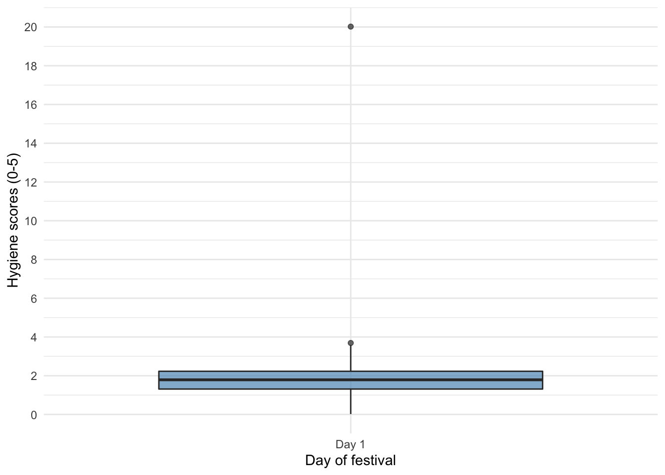
Boxplot day 1
ggplot2::ggplot(download_tib, aes(x = "Day 1", y = day_1)) +
  geom_boxplot(fill = "#5c97bf", alpha = 0.7) +
  scale_y_continuous(breaks = seq(0, 20, 2)) +
  labs(x = "Day of festival", y = "Hygiene scores (0-5)") +
  theme_minimal()
Filter the data
download_tib %>%
  dplyr::filter(day_1 > 4)
## # A tibble: 1 x 5
##   ticket_no gender day_1 day_2 day_3
##   <chr>     <fct>  <dbl> <dbl> <dbl>
## 1 4158      Female  20.0  2.44    NA
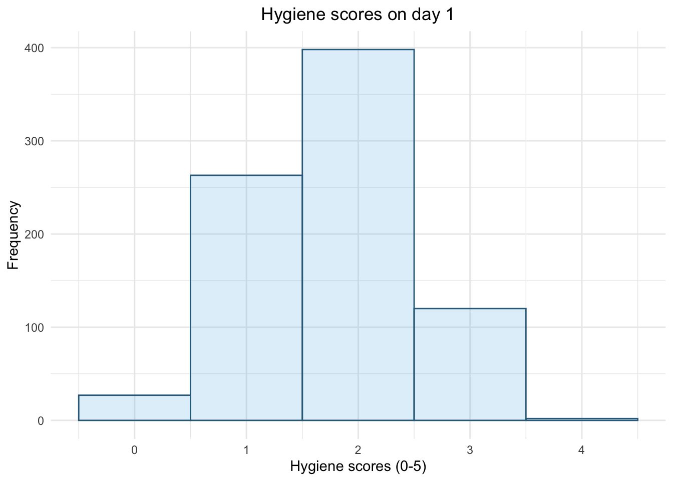
Replace the incorrect value
download_tib <- download_tib %>%
  dplyr::mutate(
    day_1 = dplyr::recode(day_1, `20.02` = 2.02)
  )
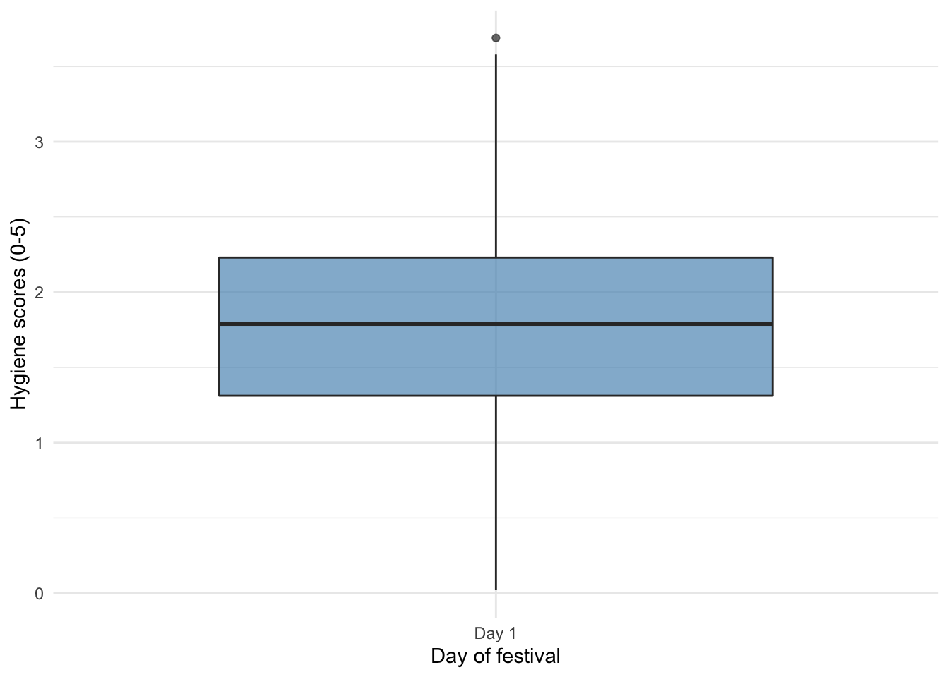
Replot the histogram and boxplot
ggplot2::ggplot(download_tib, aes(day_1)) +
  geom_histogram(binwidth = 1, fill = "#56B4E9", colour = "#336c8b", alpha = 0.2) +
  labs(y = "Frequency", x = "Hygiene scores (0-5)", title = "Hygiene scores on day 1") +
  theme_minimal() +
  theme(plot.title = element_text(hjust = 0.5))
ggplot2::ggplot(download_tib, aes(x = "Day 1", y = day_1)) +
  geom_boxplot(fill = "#5c97bf", alpha = 0.7) +
  scale_y_continuous(breaks = seq(0, 4, 1)) +
  labs(x = "Day of festival", y = "Hygiene scores (0-5)") +
  theme_minimal()
Tranforming between messy and tidy data formats
download_tidy_tib <- download_tib %>%
  tidyr::pivot_longer(
  cols = day_1:day_3,
  names_to = "day",
  values_to = "hygiene",
)
# If you want to tidy up the labels of day

download_tidy_tib <- download_tidy_tib %>%
  dplyr::mutate(
    day = stringr::str_to_sentence(day) %>%
      stringr::str_replace(., "_", " ")
  )
Converting back to messy format:
download_tib <- download_tidy_tib %>%
  tidyr::pivot_wider(
  id_cols = c(ticket_no, gender),
  names_from = "day",
  values_from = "hygiene",
)
splitting multiple variables
# Generate some random 'messy' format data

set.seed(666)
wetwipe_tib <- tibble::tibble(
  id = 1:10,
  wetwipe_day1 = round(rnorm(10, 1.7, 0.6), 2),
  wetwipe_day2 = round(rnorm(10, 1.5, 0.6), 2),
  wetwipe_day3 = round(rnorm(10, 1.5, 0.6), 2),
  none_day1 = round(rnorm(10, 1.7, 0.6), 2),
  none_day2 = round(rnorm(10, 0.8, 0.6), 2),
  none_day3 = round(rnorm(10, 0.8, 0.6), 2)
)

# Tidy that shit up ..

wetwipe_tidy_tib <- wetwipe_tib %>%
  tidyr::pivot_longer(
    cols = wetwipe_day1:none_day3,
    names_to = c("wetwipe", "day"),
    names_sep = "_",
    values_to = "hygiene"
  )

# Reverse that shit ....

wetwipe_tib <- wetwipe_tidy_tib %>%
  tidyr::pivot_wider(
    id_cols = id,
    names_from = c("wetwipe", "day"),
    names_sep = "_",
    values_from = "hygiene"
  )
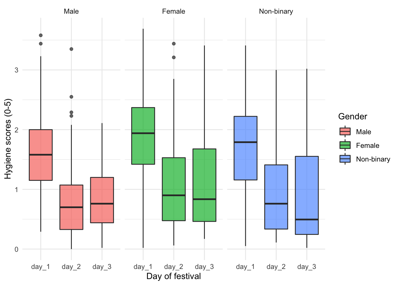
Boxplots for each day split by gender
ggplot2::ggplot(download_tidy_tib, aes(day, hygiene, fill = gender)) +
  geom_boxplot(alpha = 0.7) +
  scale_y_continuous(breaks = seq(0, 4, 1)) +
  labs(x = "Day of festival", y = "Hygiene scores (0-5)", fill = "Gender") +
  facet_wrap(~ gender) +
  theme_minimal()
Using z-scores
Manually convert to z:
make_z <- function(x){
  (x - mean(x, na.rm = TRUE)) / sd(x, na.rm = TRUE)
}

download_tib <- download_tib %>%
  dplyr::mutate(
    day_1_z = make_z(day_1),
    day_2_z = make_z(day_2),
    day_3_z = make_z(day_3)
  )

download_tib
## # A tibble: 810 x 8
##    ticket_no gender day_1 day_2  day_3 day_1_z day_2_z day_3_z
##    <chr>     <fct>  <dbl> <dbl>  <dbl>   <dbl>   <dbl>   <dbl>
##  1 2111      Male    2.64  1.35  1.61    1.25    0.540   0.892
##  2 2229      Female  0.97  1.41  0.290  -1.16    0.623  -0.967
##  3 2338      Male    0.84 NA    NA      -1.34   NA      NA
##  4 2384      Female  3.03 NA    NA       1.82   NA      NA
##  5 2401      Female  0.88  0.08 NA      -1.28   -1.22   NA
##  6 2405      Male    0.85 NA    NA      -1.33   NA      NA
##  7 2467      Female  1.56 NA    NA      -0.304  NA      NA
##  8 2478      Female  3.02 NA    NA       1.80   NA      NA
##  9 2490      Male    2.29 NA    NA       0.748  NA      NA
## 10 2504      Female  1.11  0.44  0.55   -0.953  -0.723  -0.600
## # … with 800 more rows
Using the much cooler dplyr::accross():
download_tib <- download_tib %>%
  dplyr::mutate(
    dplyr::across(day_1:day_3, list(make_z))
  )
Filter a variable at a time
download_tib %>%
  dplyr::filter(abs(day_1_z) >= 1.96) %>%
  dplyr::arrange(day_1_z)
## # A tibble: 39 x 11
##    ticket_no gender day_1  day_2 day_3 day_1_z day_2_z day_3_z day_1_1 day_2_1
##    <chr>     <fct>  <dbl>  <dbl> <dbl>   <dbl>   <dbl>   <dbl>   <dbl>   <dbl>
##  1 4107      Female 0.02  NA        NA   -2.52  NA          NA   -2.52  NA
##  2 3540      Non-b… 0.05  NA        NA   -2.48  NA          NA   -2.48  NA
##  3 2662      Female 0.11  NA        NA   -2.40  NA          NA   -2.40  NA
##  4 3030      Non-b… 0.11   0.290    NA   -2.40  -0.931      NA   -2.40  -0.931
##  5 3511      Female 0.23   0.14     NA   -2.22  -1.14       NA   -2.22  -1.14
##  6 4011      Female 0.23   0.84     NA   -2.22  -0.168      NA   -2.22  -0.168
##  7 2606      Non-b… 0.26  NA        NA   -2.18  NA          NA   -2.18  NA
##  8 4697      Male   0.290  0.14     NA   -2.14  -1.14       NA   -2.14  -1.14
##  9 3587      Male   0.3   NA        NA   -2.12  NA          NA   -2.12  NA
## 10 3260      Male   0.32  NA        NA   -2.09  NA          NA   -2.09  NA
## # … with 29 more rows, and 1 more variable: day_3_1 <dbl>
Filter by all variables:
download_tib %>%
  dplyr::filter_at(
    vars(day_1_z:day_3_z), any_vars(. >= 2.58)
    ) %>%
  dplyr::select(-c(day_1:day_3))
## # A tibble: 8 x 8
##   ticket_no gender     day_1_z day_2_z day_3_z day_1_1 day_2_1 day_3_1
##   <chr>     <fct>        <dbl>   <dbl>   <dbl>   <dbl>   <dbl>   <dbl>
## 1 3374      Male          2.61    3.31   NA       2.61    3.31   NA
## 2 3787      Non-binary    1.99    2.83   NA       1.99    2.83   NA
## 3 3828      Female        2.23    3.12   NA       2.23    3.12   NA
## 4 4016      Female        2.77   NA      NA       2.77   NA      NA
## 5 4165      Female        1.51    2.29    2.88    1.51    2.29    2.88
## 6 4172      Non-binary    2.23    2.70    2.88    2.23    2.70    2.88
## 7 4564      Female        2.32    3.44    3.43    2.32    3.44    3.43
## 8 4590      Female        2.07    2.62   NA       2.07    2.62   NA
get_cum_percent <- function(var,  cut_off = 1.96){
  ecdf_var <- abs(var) %>% ecdf()
  100*(1 - ecdf_var(cut_off))
}

download_tib %>%
  dplyr::summarize(
    `z >= 1.96` = get_cum_percent(day_1_z),
    `z >= 2.58` = get_cum_percent(day_1_z,cut_off = 2.58),
    `z >= 3.29` = get_cum_percent(day_1_z,cut_off = 3.29)
  )
## # A tibble: 1 x 3
##   `z >= 1.96` `z >= 2.58` `z >= 3.29`
##         <dbl>       <dbl>       <dbl>
## 1        4.81       0.247           0
download_tidy_tib <- download_tidy_tib %>%
  group_by(day) %>%
  dplyr::mutate(
    zhygiene = make_z(hygiene)
  )


download_tidy_tib %>%
  group_by(day) %>%
  dplyr::summarize(
    `z >= 1.96` = get_cum_percent(zhygiene),
    `z >= 2.58` = get_cum_percent(zhygiene,cut_off = 2.58),
    `z >= 3.29` = get_cum_percent(zhygiene,cut_off = 3.29)
  )
## # A tibble: 3 x 4
##   day   `z >= 1.96` `z >= 2.58` `z >= 3.29`
##   <chr>       <dbl>       <dbl>       <dbl>
## 1 day_1        4.81       0.247       0
## 2 day_2        6.82       2.27        0.758
## 3 day_3        4.07       2.44        0.813
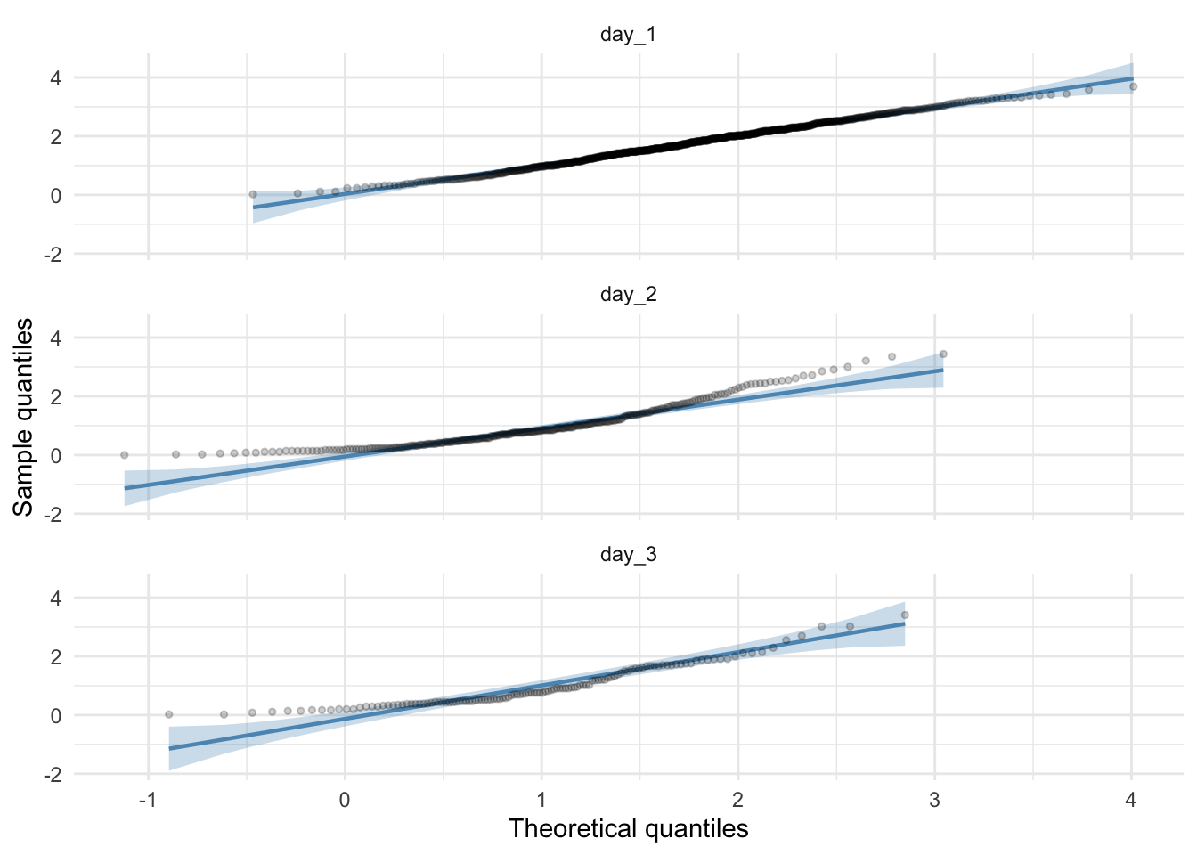
Q-Q plots
Standard Q-Q plot of the hygiene scores
download_tidy_tib %>%
  ggplot2::ggplot(., aes(sample = hygiene)) +
  qqplotr::stat_qq_band(fill = "#5c97bf", alpha = 0.3) +
  qqplotr::stat_qq_line(colour = "#5c97bf") +
  qqplotr::stat_qq_point(alpha = 0.2, size = 1) +
  labs(x = "Theoretical quantiles", y = "Sample quantiles") +
  facet_wrap(~day, ncol = 1) +
  theme_minimal()
Detrended Q-Q plot
download_tidy_tib %>%
  dplyr::filter(day == "Day 2") %>%
  ggplot2::ggplot(., aes(sample = hygiene)) +
  qqplotr::stat_qq_band(fill = "#5c97bf", alpha = 0.3, detrend = TRUE) +
  qqplotr::stat_qq_line(colour = "#5c97bf", detrend = TRUE) +
  qqplotr::stat_qq_point(alpha = 0.2, size = 1, detrend = TRUE) +
  labs(x = "Theoretical quantiles", y = "Sample quantiles") +
  theme_minimal()
Skew and kurtosis
download_tidy_tib %>%
  dplyr::group_by(day) %>%
  dplyr::summarize(
    valid_cases = sum(!is.na(hygiene)),
    mean = ggplot2::mean_cl_normal(hygiene)$y,
    ci_lower = ggplot2::mean_cl_normal(hygiene)$ymin,
    ci_upper = ggplot2::mean_cl_normal(hygiene)$ymax,
    skew = moments::skewness(hygiene, na.rm = TRUE),
    kurtosis = moments::kurtosis(hygiene, na.rm = TRUE)
  )
## # A tibble: 3 x 7
##   day   valid_cases  mean ci_lower ci_upper     skew kurtosis
##   <chr>       <int> <dbl>    <dbl>    <dbl>    <dbl>    <dbl>
## 1 day_1         810 1.77     1.72      1.82 -0.00444     2.58
## 2 day_2         264 0.961    0.874     1.05  1.09        3.78
## 3 day_3         123 0.977    0.850     1.10  1.02        3.65
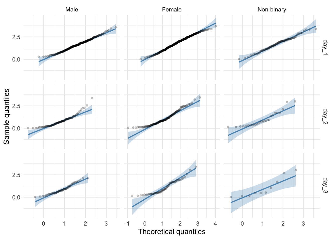
Splitting by gender
download_tidy_tib %>%
  dplyr::group_by(gender, day) %>%
  dplyr::summarize(
    valid_cases = sum(!is.na(hygiene)),
    mean = ggplot2::mean_cl_normal(hygiene)$y,
    ci_lower = ggplot2::mean_cl_normal(hygiene)$ymin,
    ci_upper = ggplot2::mean_cl_normal(hygiene)$ymax,
    skew = moments::skewness(hygiene, na.rm = TRUE),
    kurtosis = moments::kurtosis(hygiene, na.rm = TRUE)
  )
## # A tibble: 9 x 8
## # Groups:   gender [3]
##   gender     day   valid_cases  mean ci_lower ci_upper    skew kurtosis
##   <fct>      <chr>       <int> <dbl>    <dbl>    <dbl>   <dbl>    <dbl>
## 1 Male       day_1         277 1.61     1.53     1.68   0.204      2.87
## 2 Male       day_2          94 0.789    0.665    0.912  1.46       6.01
## 3 Male       day_3          53 0.855    0.705    1.00   0.636      2.56
## 4 Female     day_1         443 1.88     1.82     1.95  -0.167      2.56
## 5 Female     day_2         143 1.08     0.953    1.20   0.839      3.05
## 6 Female     day_3          60 1.08     0.879    1.27   0.887      3.22
## 7 Non-binary day_1          90 1.72     1.56     1.88  -0.0165     2.66
## 8 Non-binary day_2          27 0.942    0.624    1.26   1.22       3.67
## 9 Non-binary day_3          10 1.03     0.247    1.81   0.920      2.31
download_tidy_tib %>%
  ggplot2::ggplot(., aes(sample = hygiene)) +
  qqplotr::stat_qq_band(fill = "#5c97bf", alpha = 0.3) +
  qqplotr::stat_qq_line(colour = "#5c97bf") +
  qqplotr::stat_qq_point(alpha = 0.2, size = 1) +
  labs(x = "Theoretical quantiles", y = "Sample quantiles") +
  facet_grid(day~gender, scales = "free_x") +
  theme_minimal()