R code Chapter 5
This document contains abridged sections from Discovering Statistics Using R and RStudio by Andy Field so there are some copyright considerations. You can use this material for teaching and non-profit activities but please do not meddle with it or claim it as your own work. See the full license terms at the bottom of the page.
Load packages
Remember to load the tidyverse:
library(tidyverse)
Load the data
Remember to install the package with library(discovr). After which you can load data into a tibble by executing:
name_of_tib <- discovr::name_of_data
For example, execute these lines to create the tibbles referred to in the chapter:
cat_tib <- discovr::catterplot
exam_tib <- discovr::exam_anxiety
grammar_tib <- discovr::social_media
notebook_tib <- discovr::notebook
hiccups_tib <- discovr::hiccups
ong_tib <- discovr::ong_tidy
wish_tib <- discovr::jiminy_cricket
If you want to read the file from the CSV and you have set up your project folder as I suggest in Chapter 1, then the general format of the code you would use is:
tibble_name <- here::here("../data/name_of_file.csv") %>%
  readr::read_csv() %>%
  dplyr::mutate(
    ...
    code to convert character variables to factors
    ...
  )
In which you’d replace tibble_name with the name you want to assign to the tibble and change name_of_file.csv to the name of the file that you’re trying to load. You can use mutate to convert categorical variables to factors. For example, for the notebook data you would load it by executing:
library(here)

notebook_tib <- here::here("data/notebook.csv") %>%
  readr::read_csv() %>%
  dplyr::mutate(
    sex = forcats::as_factor(sex),
    film = forcats::as_factor(film)
  )
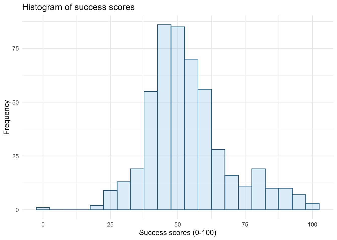
Histograms
ggplot2::ggplot(wish_tib, aes(success)) +
 geom_histogram(binwidth = 5, fill = "#56B4E9", colour = "#336c8b", alpha = 0.2) +
 labs(y = "Frequency", x = "Success scores (0-100)", title = "Histogram of success scores") +
 theme_minimal()
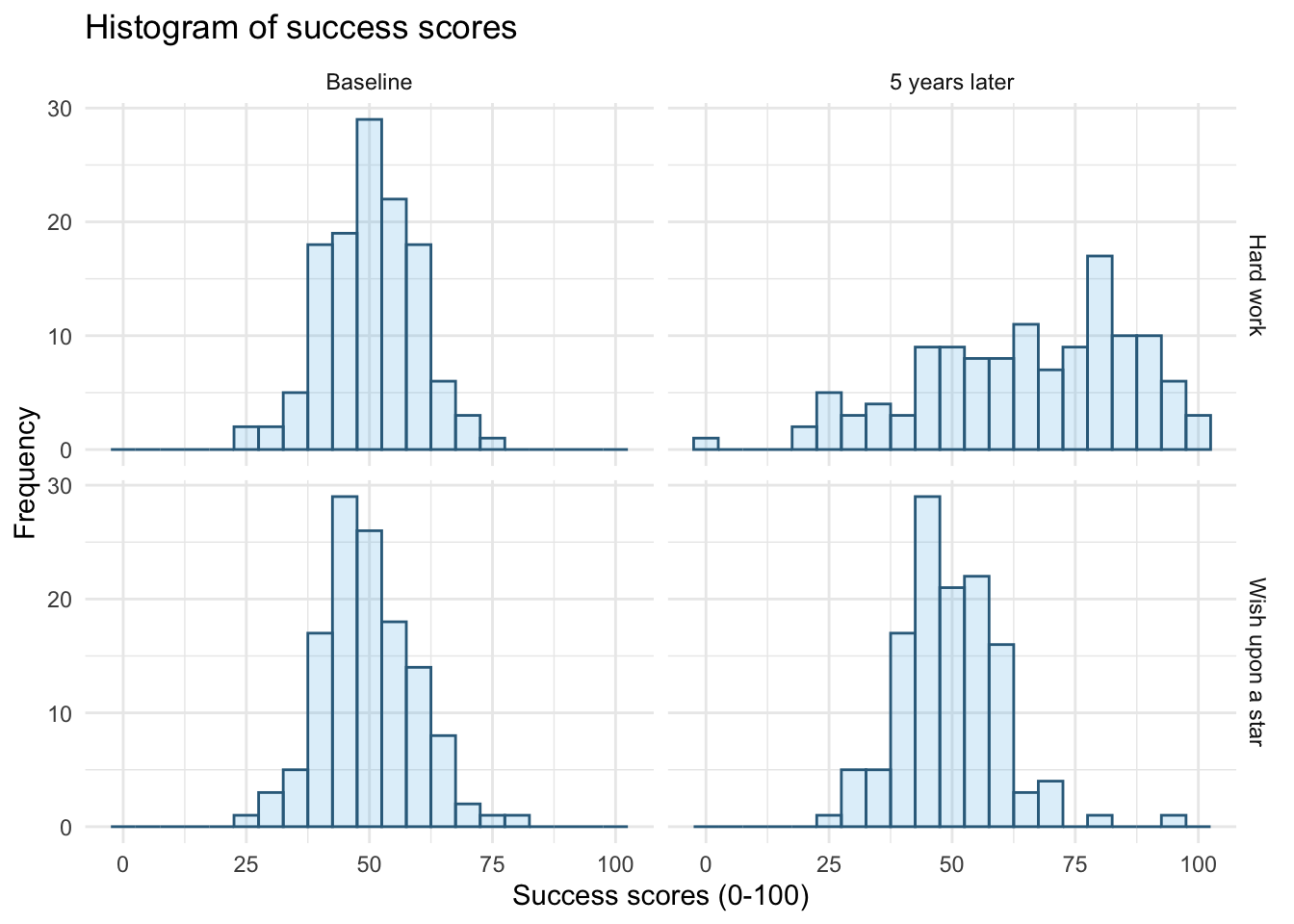
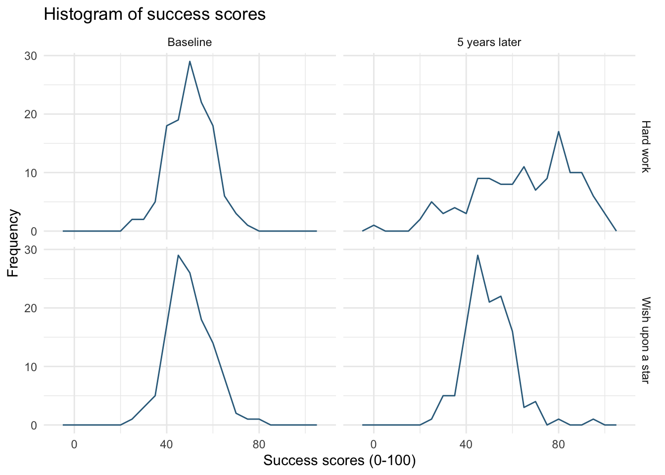
ggplot2::ggplot(wish_tib, aes(success)) +
 geom_histogram(binwidth = 5, fill = "#56B4E9", colour = "#336c8b", alpha = 0.2) +
 labs(y = "Frequency", x = "Success scores (0-100)", title = "Histogram of success scores") +
 facet_grid(strategy~time) +
 theme_minimal()
Frequency polygon
ggplot2::ggplot(wish_tib, aes(success)) +
 geom_freqpoly(binwidth = 5, colour = "#336c8b") +
 labs(y = "Frequency", x = "Success scores (0-100)", title = "Histogram of success scores") +
 facet_grid(strategy~time) +
 theme_minimal()
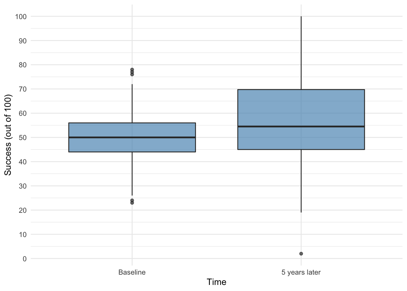
Boxplots
ggplot2::ggplot(wish_tib, aes(time, success)) +
  geom_boxplot(fill = "#5c97bf", alpha = 0.7) +
  scale_y_continuous(breaks = seq(0, 100, 10)) +
  labs(x = "Time", y = "Success (out of 100)") +
  theme_minimal()
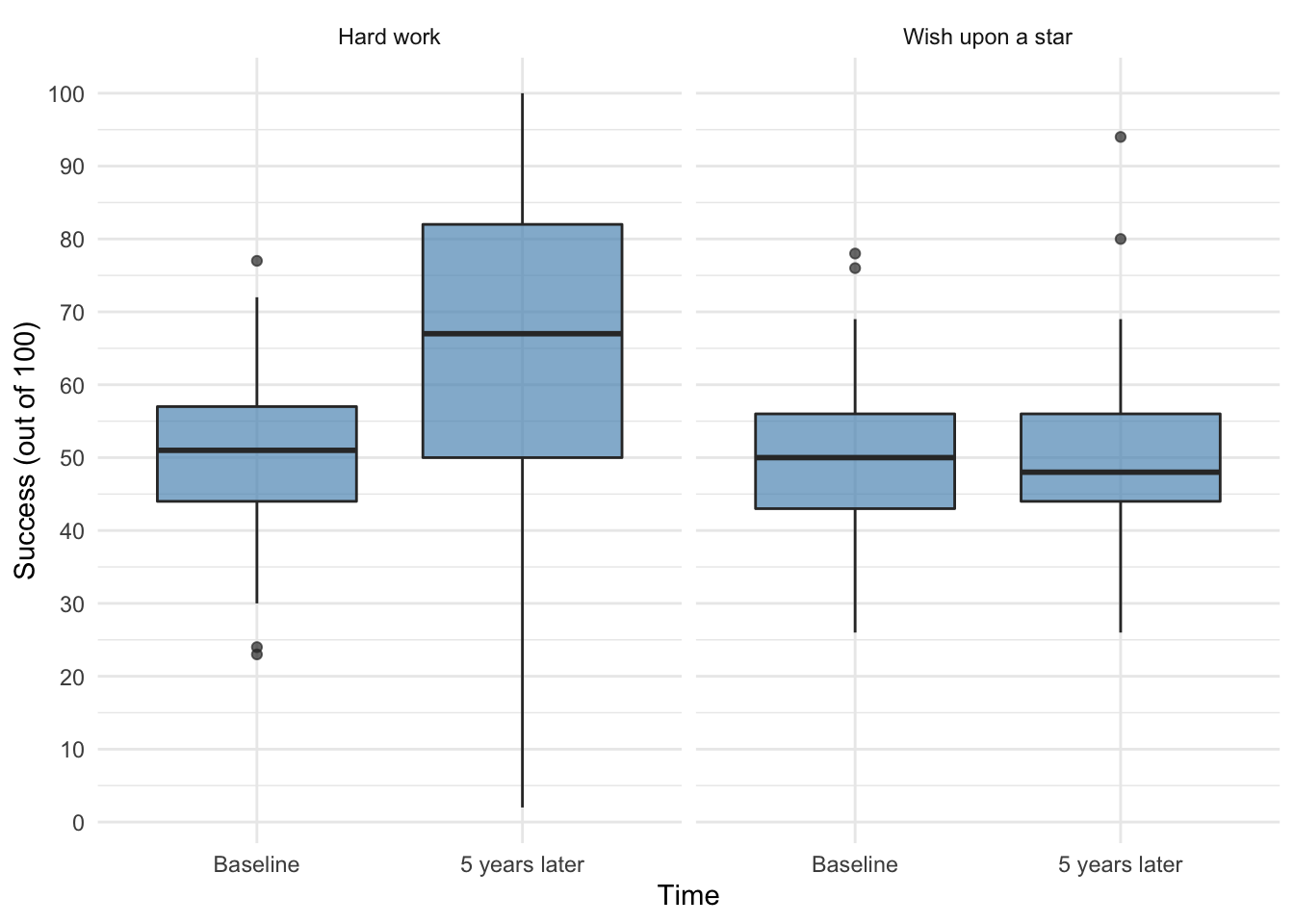
ggplot2::ggplot(wish_tib, aes(time, success)) +
  geom_boxplot(fill = "#5c97bf", alpha = 0.7) +
  scale_y_continuous(breaks = seq(0, 100, 10)) +
  labs(x = "Time", y = "Success (out of 100)") +
  facet_wrap(~ strategy) +
  theme_minimal()
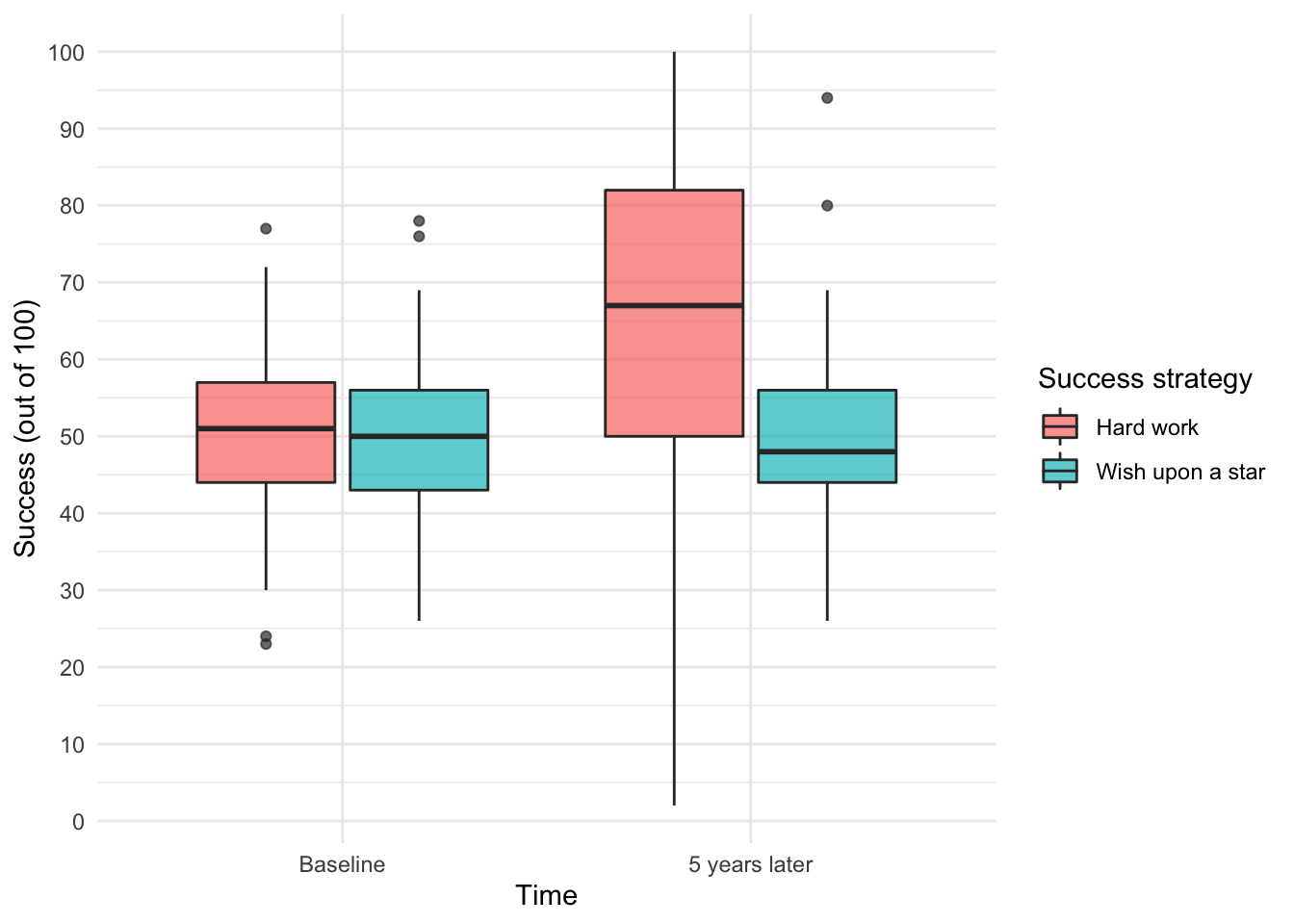
ggplot2::ggplot(wish_tib, aes(time, success, fill = strategy)) +
  geom_boxplot(alpha = 0.7) +
  scale_y_continuous(breaks = seq(0, 100, 10)) +
  labs(x = "Time", y = "Success (out of 100)", fill = "Success strategy") +
  theme_minimal()
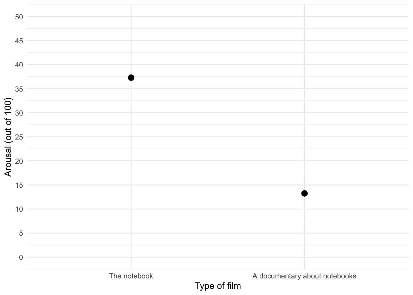
Plotting means
note_mean  <- ggplot2::ggplot(notebook_tib, aes(film, arousal))
note_mean +
  stat_summary(fun = "mean", geom = "point", size = 3)+
  coord_cartesian(ylim = c(0, 50)) +
  scale_y_continuous(breaks = seq(0, 50, 5)) +
  labs(x = "Type of film", y = "Arousal (out of 100)") +
  theme_minimal()
`
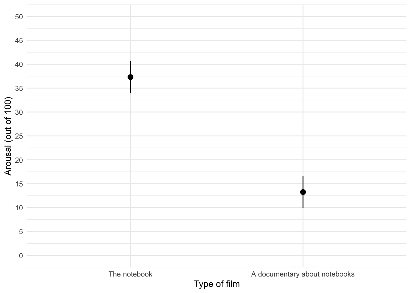
note_mean +
  stat_summary(fun.data = "mean_cl_normal", geom = "pointrange") +
  coord_cartesian(ylim = c(0, 50)) +
  scale_y_continuous(breaks = seq(0, 50, 5)) +
  labs(x = "Type of film", y = "Arousal (out of 100)") +
  theme_minimal()
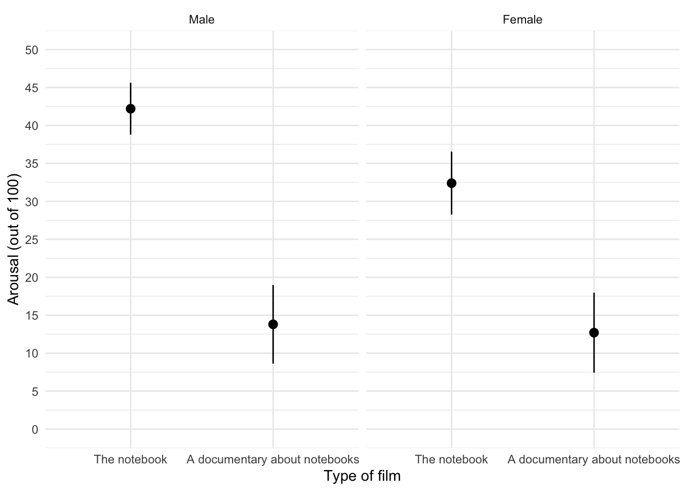
ggplot2::ggplot(notebook_tib, aes(film, arousal)) +
  stat_summary(fun.data = "mean_cl_normal", geom = "pointrange") +
  coord_cartesian(ylim = c(0, 50)) +
  scale_y_continuous(breaks = seq(0, 50, 5)) +
  labs(x = "Type of film", y = "Arousal (out of 100)") +
  facet_wrap(~sex) +
  theme_minimal()
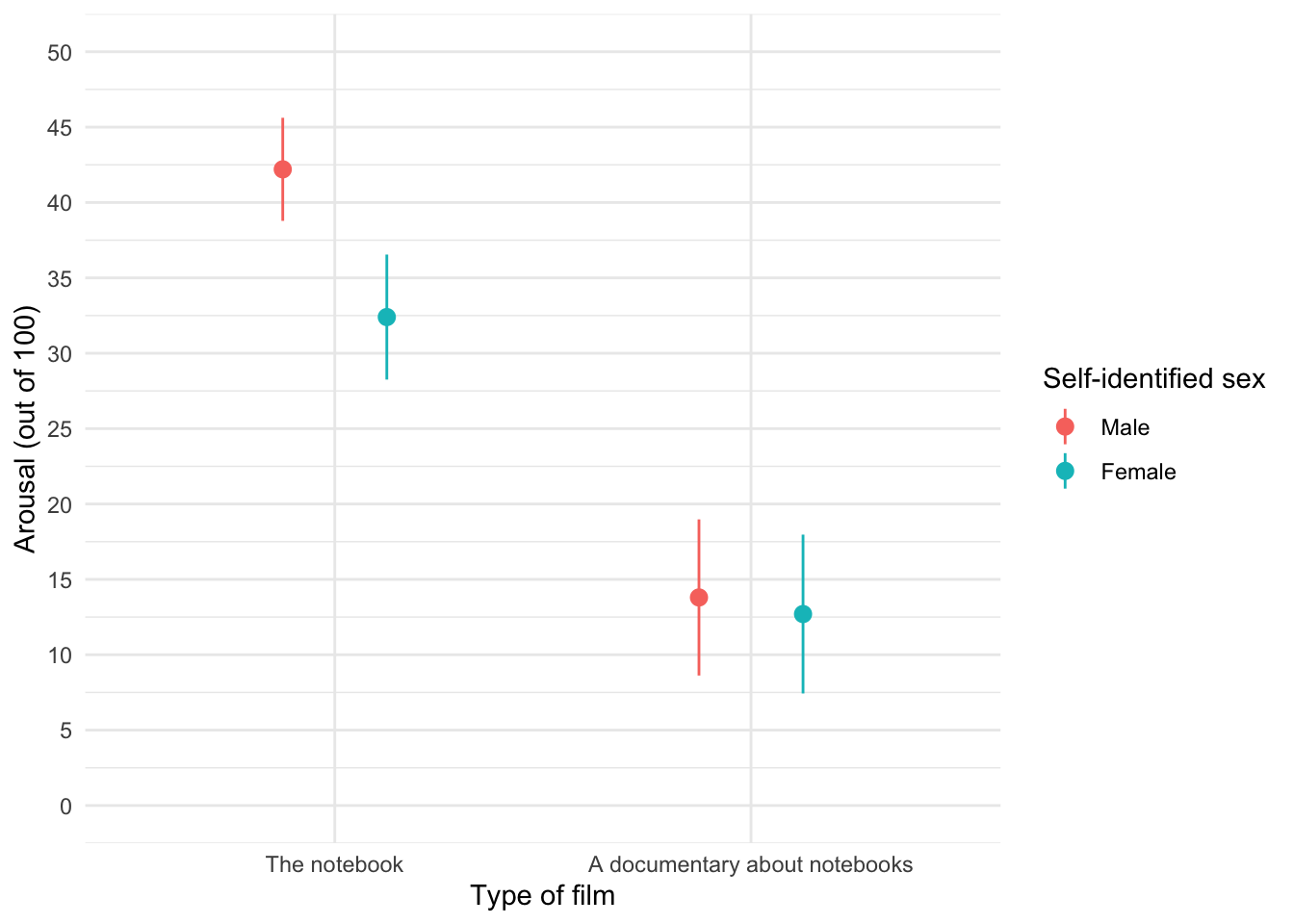
ggplot2::ggplot(notebook_tib, aes(film, arousal, colour = sex)) +
  stat_summary(fun.data = "mean_cl_normal", geom = "pointrange", position = position_dodge(width = 0.5)) +
  coord_cartesian(ylim = c(0, 50)) +
  scale_y_continuous(breaks = seq(0, 50, 5)) +
  labs(x = "Type of film", y = "Arousal (out of 100)", colour = "Self-identified sex") +
  theme_minimal()
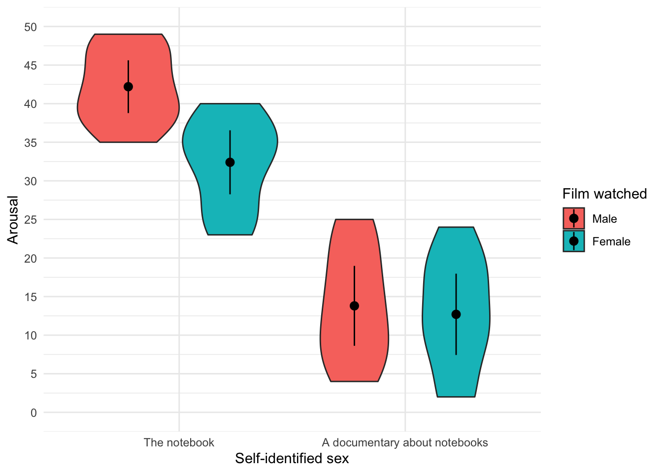
Violin plots
ggplot2::ggplot(notebook_tib, aes(film, arousal, fill = sex)) +
  geom_violin() +
  stat_summary(fun.data = "mean_cl_normal", geom = "pointrange", position = position_dodge(width = 0.9)) +
  labs(x = "Self-identified sex", y = "Arousal", fill = "Film watched") +
  coord_cartesian(ylim = c(0, 50)) +
  scale_y_continuous(breaks = seq(0, 50, 5)) +
  theme_minimal()
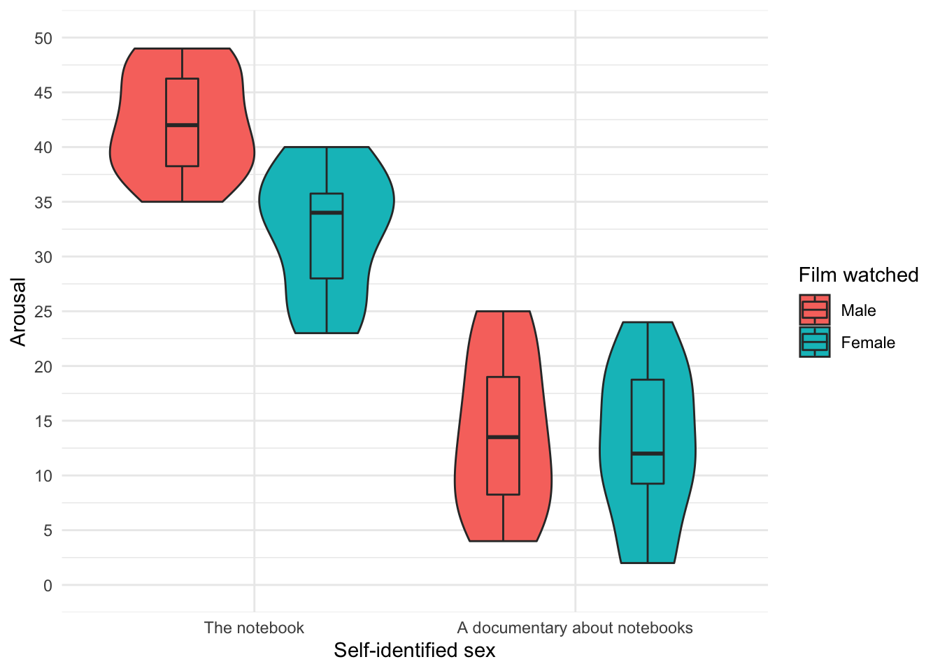
ggplot2::ggplot(notebook_tib, aes(film, arousal, fill = sex)) +
  geom_violin() +
  geom_boxplot(width = 0.2, position = position_dodge(width = 0.9)) +
  labs(x = "Self-identified sex", y = "Arousal", fill = "Film watched") +
  coord_cartesian(ylim = c(0, 50)) +
  scale_y_continuous(breaks = seq(0, 50, 5)) +
  theme_minimal()
Repeated measures
hiccups_tib %>%
  dplyr::arrange(id)
## # A tibble: 60 x 3
##    id    intervention hiccups
##    <chr> <fct>          <dbl>
##  1 djgu  Baseline           7
##  2 djgu  Tongue            15
##  3 djgu  Carotid           10
##  4 djgu  Rectum             5
##  5 dtht  Baseline           3
##  6 dtht  Tongue            14
##  7 dtht  Carotid           11
##  8 dtht  Rectum             4
##  9 ehv   Baseline          13
## 10 ehv   Tongue            18
## # … with 50 more rows
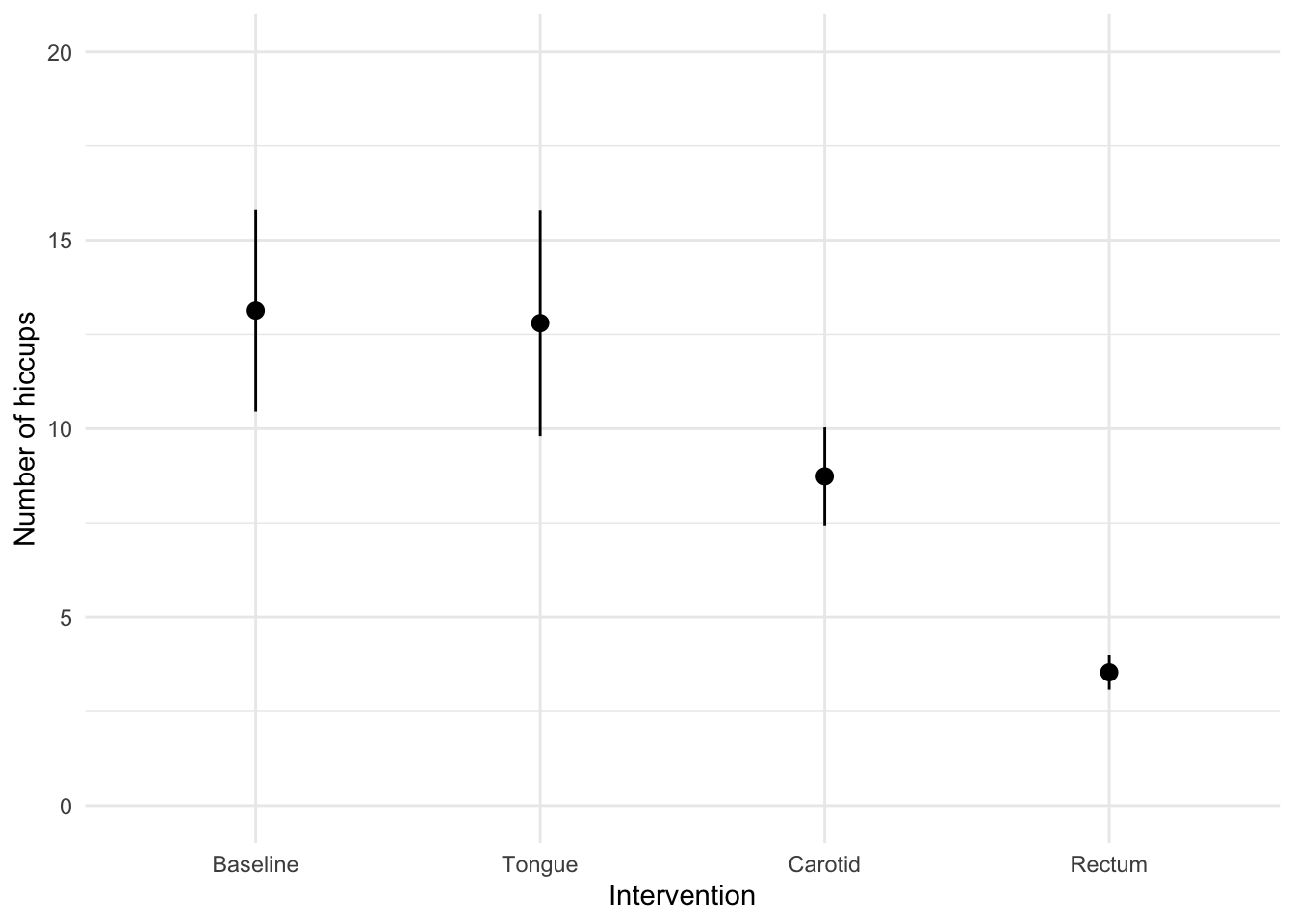
ggplot2::ggplot(hiccups_tib, aes(intervention, hiccups)) +
  stat_summary(fun.data = "mean_cl_normal", geom = "pointrange") +
  labs(x = "Intervention", y = "Number of hiccups") +
  coord_cartesian(ylim = c(0, 20)) +
  scale_y_continuous(breaks = seq(0, 20, 5)) +
  theme_minimal()
Line plots and mixed designs
grammar_tib %>%
  dplyr::arrange(id)
## # A tibble: 100 x 4
##    id    media_use  time     grammar
##    <chr> <fct>      <fct>      <dbl>
##  1 ajlx  Banned     Baseline      75
##  2 ajlx  Banned     6 months      70
##  3 ajot  Banned     Baseline      54
##  4 ajot  Banned     6 months      74
##  5 aorr  Encouraged Baseline      51
##  6 aorr  Encouraged 6 months      60
##  7 awrx  Banned     Baseline      66
##  8 awrx  Banned     6 months      55
##  9 axun  Encouraged Baseline      77
## 10 axun  Encouraged 6 months      61
## # … with 90 more rows
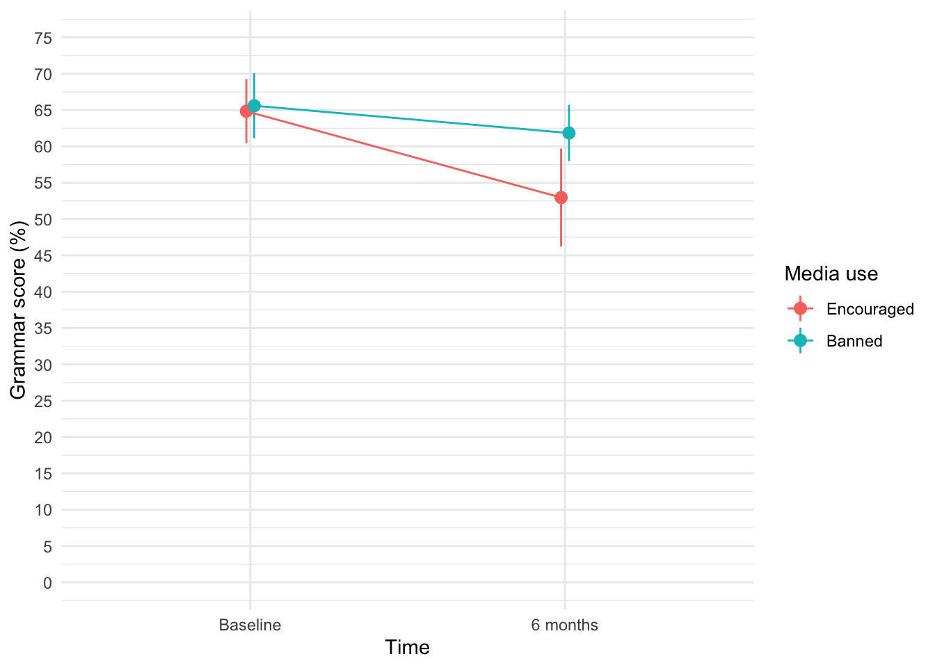
ggplot2::ggplot(grammar_tib, aes(time, grammar, colour = media_use)) +
  stat_summary(fun.data = "mean_cl_normal", geom = "pointrange", position = position_dodge(width = 0.05)) +
  stat_summary(fun = "mean", geom = "line", position = position_dodge(width = 0.05), aes(group = media_use)) +
  labs(x = "Time", y = "Grammar score (%)", colour = "Media use") +
  coord_cartesian(ylim = c(0, 75)) +
  scale_y_continuous(breaks = seq(0, 75, 5)) +
  theme_minimal()
Scatterplots
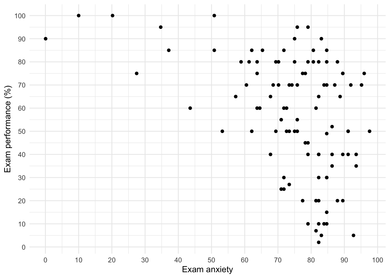
Simple scatterplot
ggplot(exam_tib, aes(anxiety, exam_grade)) +
  geom_point() +
  labs(x = "Exam anxiety", y = "Exam performance (%)") +
  scale_y_continuous(breaks = seq(0, 100, 10)) +
  scale_x_continuous(breaks = seq(0, 100, 10)) +
  theme_minimal()
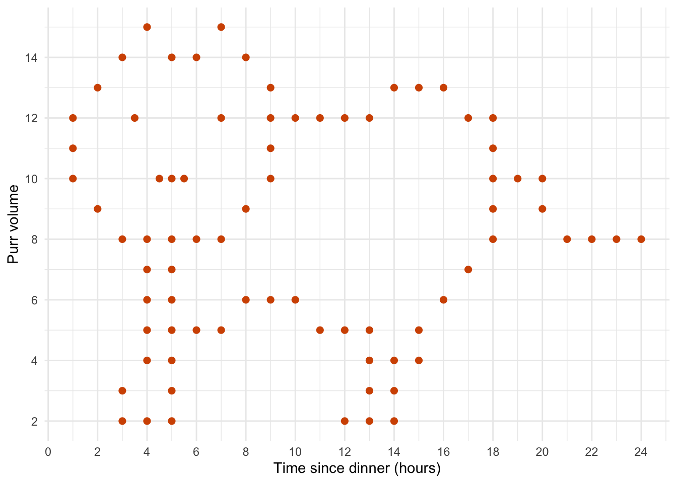
Catterplots
ggplot(cat_tib, aes(dinner_time, meow)) +
  geom_point(colour = "#d35400", size = 2) +
  scale_y_continuous(breaks = seq(0, 16, 2)) +
  scale_x_continuous(breaks = seq(0, 24, 2)) +
  labs(x = "Time since dinner (hours)", y = "Purr volume") +
  theme_minimal()
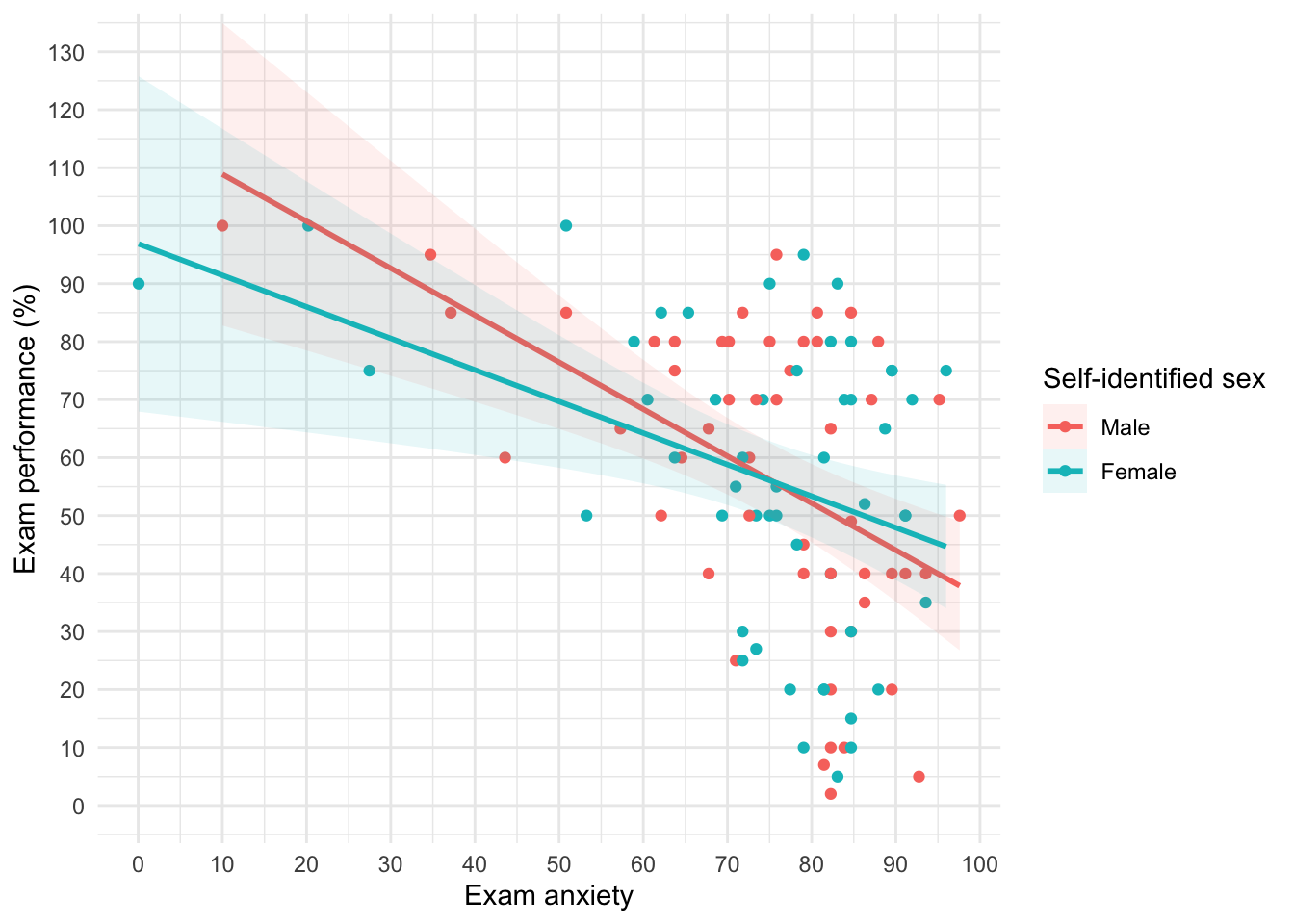
Grouped scatterplots
ggplot(exam_tib, aes(anxiety, exam_grade, colour = sex))  +
  geom_point() +
  geom_smooth(method = "lm", aes(fill = sex), alpha = 0.1) +
  labs(x = "Exam anxiety", y = "Exam performance (%)", colour = "Self-identified sex", fill = "Self-identified sex") +
  coord_cartesian(ylim = c(0, 130)) +
  scale_y_continuous(breaks = seq(0, 130, 10)) +
  scale_x_continuous(breaks = seq(0, 100, 10)) +
  theme_minimal()
## `geom_smooth()` using formula 'y ~ x'
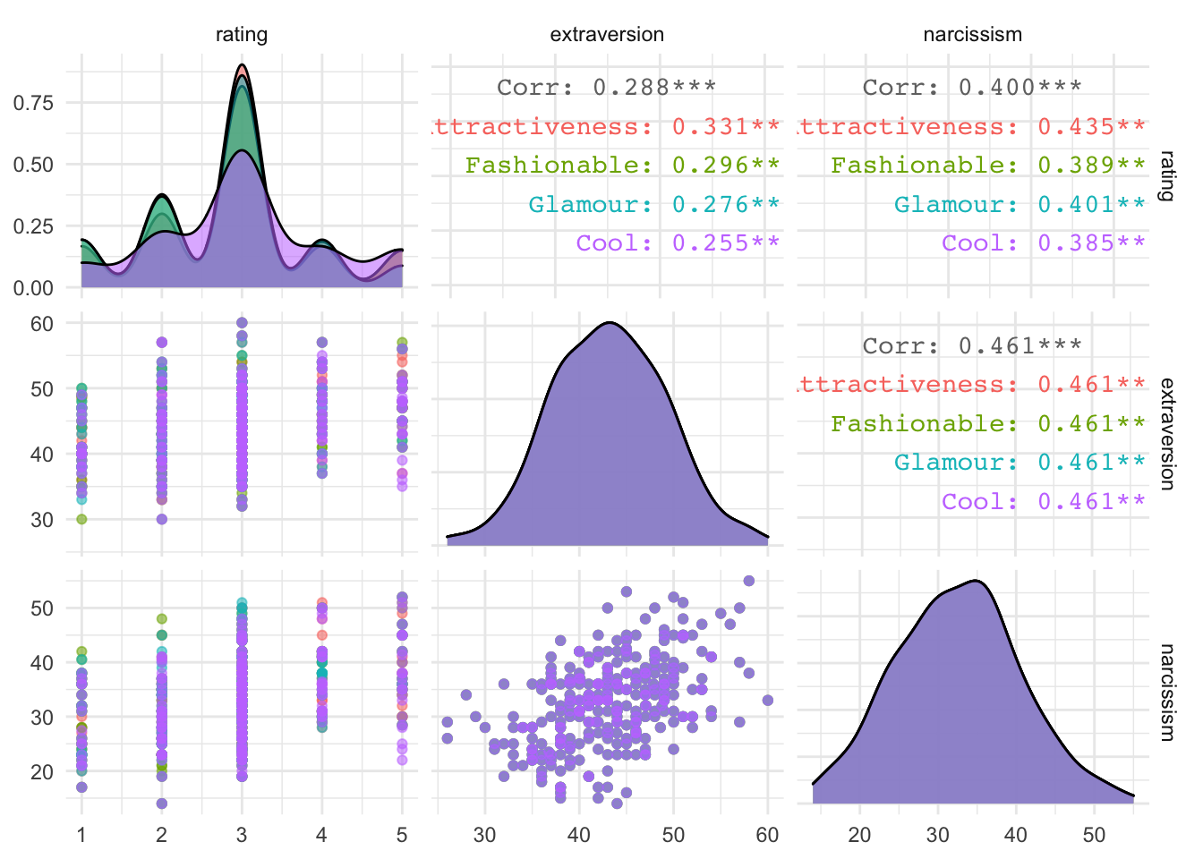
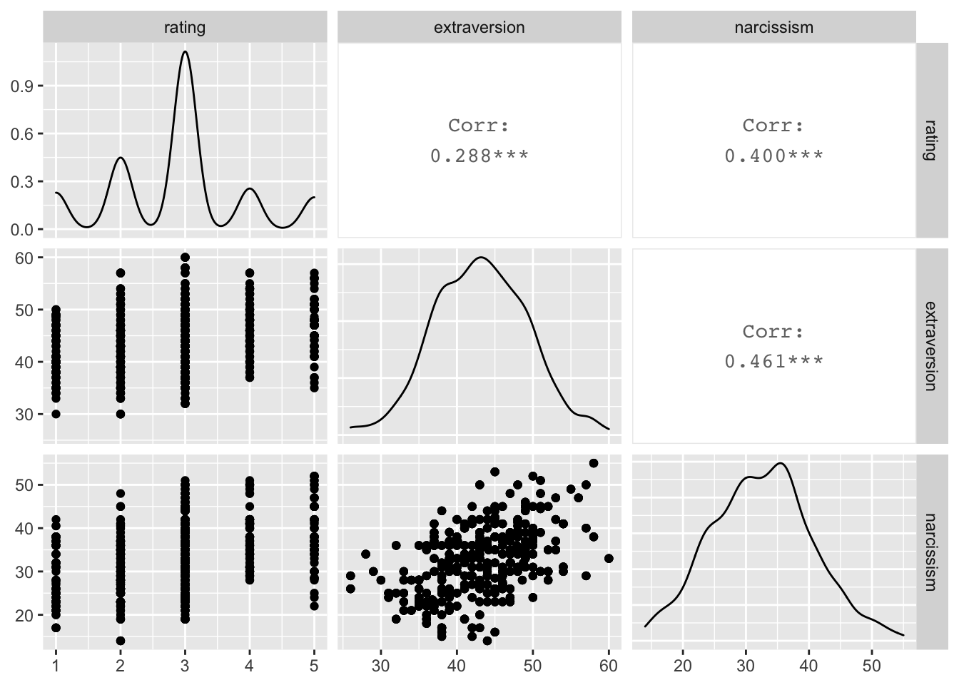
Matrix scatterplots
GGally::ggpairs(ong_tib, columns = c("rating", "extraversion", "narcissism"))
## Registered S3 method overwritten by 'GGally':
##   method from
##   +.gg   ggplot2
## Warning: Removed 324 rows containing non-finite values (stat_density).
## Warning in ggally_statistic(data = data, mapping = mapping, na.rm = na.rm, :
## Removed 324 rows containing missing values

## Warning in ggally_statistic(data = data, mapping = mapping, na.rm = na.rm, :
## Removed 324 rows containing missing values
## Warning: Removed 324 rows containing missing values (geom_point).

## Warning: Removed 324 rows containing missing values (geom_point).
GGally::ggpairs(ong_tib, columns = c("rating", "extraversion", "narcissism"), mapping = aes(colour = rating_type, alpha = 0.1)) + theme_minimal()
## Warning: Removed 324 rows containing non-finite values (stat_density).
## Warning in ggally_statistic(data = data, mapping = mapping, na.rm = na.rm, :
## Removed 324 rows containing missing values

## Warning in ggally_statistic(data = data, mapping = mapping, na.rm = na.rm, :
## Removed 324 rows containing missing values
## Warning: Removed 324 rows containing missing values (geom_point).

## Warning: Removed 324 rows containing missing values (geom_point).