Smart Alex solutions Chapter 18

Task 18.1
Rerun the analysis in this chapter using principal component analysis and compare the results to those in the chapter.
Load the data
To load the data from the CSV file (assuming you have set up a project folder as suggested in the book):
raq_tib <- here::here("data/raq.csv") %>%
  readr::read_csv()
Alternative, load the data directly from the discovr package:
raq_tib <- discovr::raq
Fit the model
All of the descriptives, correlation matrices, KMO tests and so on are unaffected by our choice of principal components as the method of dimension reduction. Also in the book chapter we did parallel analysis based on components and this suggested 4 components (as did the parallel analysis based on components). So, follow everything in the book (code and interpretation) up to the point at which we for the main model.
As a reminder, we set up the correlation matrix to be based on polychoric correlations
# create tibble that contains only the questionnaire items
raq_items_tib <- raq_tib %>%
  dplyr::select(-id)
# get the polychoric correlation object
raq_poly <- psych::polychoric(raq_items_tib)
# store the polychoric correlation matrix
raq_cor <- raq_poly$rho
Things start to get different at the point of fitting the model. We can use the same code as the book chapter except that we use the pca() (or principal() if you prefer) function instead of fa() and we need to remove scores = "tenBerge" because for PCA there is only a single method for computing component scores (and this is used by default). We also need to add rotate = "oblimin" because for PCA the default is to use an orthogonal rotation (varimax). I’ve also changed the name of the object to store this in to raq_pca to reflect the fact we’ve done PCA and not component analysis.
From the raw data:
raq_pca <- psych::pca(raq_items_tib,
                    nfactors = 4,
                    cor = "poly",
                    rotate = "oblimin"
                    )
From the correlation matrix:
raq_pca <- psych::pca(raq_cor,
                    n.obs = 2571,
                    nfactors = 4,
                    rotate = "oblimin"
                    )
To see the output:
raq_pca
Note that the components are labelled TC1 to TC4 (unlike for the component analysis in the book where the labels were MR1 etc.). We are given some information about how much variance each component accounts for.
##                        TC1  TC2  TC3  TC4
## SS loadings           3.67 2.77 2.60 2.32
## Proportion Var        0.16 0.12 0.11 0.10
## Cumulative Var        0.16 0.28 0.39 0.49
## Proportion Explained  0.32 0.24 0.23 0.20
## Cumulative Proportion 0.32 0.57 0.80 1.00
We see, for example, from Proportion Var that TC1 accounts for 0.16 of the overall variance (16%) and TC2 accounts for 0.12 of the variance (12%) and so on. The Cumulative Var is the proportion of variance explained cumulatively by the components. So, cumulatively, TC1 accounts for 0.16 of the overall variance (16%) and TC1 and TC2 together account for 0.16 + 0.12 = 0.28 of the variance (28%). Importantly, we can see that all four components in combination explain 0.49 of the overall variance (49%).
The Proportion Explained is the proportion of the explained variance, that is explained by a component. So, of the 49% of variance accounted for, 0.32 (32%) is attributable to TC1, 0.25 (25%) to TC2, 0.24 (24%) to TC3 and 0.19 (19%) to TC4.
##
## Factor analysis with Call: principal(r = r, nfactors = nfactors, residuals = residuals,
##     rotate = rotate, n.obs = n.obs, covar = covar, scores = scores,
##     missing = missing, impute = impute, oblique.scores = oblique.scores,
##     method = method, use = use, cor = cor, correct = 0.5, weight = NULL)
##
## Test of the hypothesis that 4 factors are sufficient.
## The degrees of freedom for the model is 167  and the objective function was  0.63
## The number of observations was  2571  with Chi Square =  1614.3  with prob <  4.9e-235
##
## The root mean square of the residuals (RMSA) is  0.05
##
##  With component correlations of
##      TC1  TC2  TC3  TC4
## TC1 1.00 0.34 0.38 0.41
## TC2 0.34 1.00 0.21 0.25
## TC3 0.38 0.21 1.00 0.41
## TC4 0.41 0.25 0.41 1.00
The correlations between components are also displayed. These are all non-zero indicating that components are correlated (and oblique rotation was appropriate). It also tells us the degree to which components are correlated. All of the components positively, and fairly strongly, correlate with each other. In other words, the latent constructs represented by the components are related.
In terms of fit
- The chi-square statistic is $ \chi^2 = $ 1614.3, p < 0.001. This is consistent with when we ran the analysis as factor analysis in the chapter.
- The RMSR is 0.05.
Let’s look at the loadings (I’ve suppressed values below 0.2 and sorted).
parameters::model_parameters(raq_pca, threshold = 0.2, sort = TRUE) %>%
  kableExtra::kable(digits = 2)
| Variable | TC1 | TC2 | TC3 | TC4 | Complexity | Uniqueness |
|---|---|---|---|---|---|---|
| raq\_06 | 0.80 | 1.02 | 0.29 | |||
| raq\_18 | 0.69 | 1.03 | 0.49 | |||
| raq\_13 | 0.68 | 1.02 | 0.56 | |||
| raq\_07 | 0.65 | 1.01 | 0.56 | |||
| raq\_10 | 0.63 | 1.09 | 0.63 | |||
| raq\_15 | 0.58 | 1.02 | 0.63 | |||
| raq\_14 | 0.53 | 1.03 | 0.70 | |||
| raq\_05 | 0.50 | 0.36 | 1.86 | 0.42 | ||
| raq\_23 | 0.86 | 1.03 | 0.31 | |||
| raq\_09 | 0.86 | 1.03 | 0.30 | |||
| raq\_19 | 0.24 | 0.65 | 1.27 | 0.41 | ||
| raq\_22 | 0.62 | 1.16 | 0.48 | |||
| raq\_02 | 0.24 | 0.59 | 1.36 | 0.52 | ||
| raq\_16 | 0.63 | 1.02 | 0.63 | |||
| raq\_04 | 0.62 | 1.03 | 0.58 | |||
| raq\_21 | 0.59 | 1.13 | 0.53 | |||
| raq\_12 | 0.58 | -0.21 | 1.26 | 0.72 | ||
| raq\_20 | 0.56 | 1.09 | 0.60 | |||
| raq\_03 | -0.54 | 1.01 | 0.70 | |||
| raq\_01 | 0.51 | 1.06 | 0.72 | |||
| raq\_08 | 0.84 | 1.01 | 0.24 | |||
| raq\_11 | 0.83 | 1.00 | 0.30 | |||
| raq\_17 | 0.83 | 1.00 | 0.33 |
The clusters of items match the book chapter where we used factor analysis instead of PCA. The questions that load highly on TC1 seem to be items that relate to Fear of computers:
- raq_05: I don’t understand statistics
- raq_06: I have little experience of computers
- raq_07: All computers hate me
- raq_10: Computers are useful only for playing games
- raq_13: I worry that I will cause irreparable damage because of my incompetence with computers
- raq_14: Computers have minds of their own and deliberately go wrong whenever I use them
- raq_15: Computers are out to get me
- raq_18: R always crashes when I try to use it
Note that item 5 also loads highly onto TC3.
The questions that load highly on TC2 seem to be items that relate to Fear of peer/social evaluation:
- raq_02: My friends will think I’m stupid for not being able to cope with {{< icon name=“r-project” pack=“fab” >}}
- raq_09: My friends are better at statistics than me
- raq_19: Everybody looks at me when I use {{< icon name=“r-project” pack=“fab” >}}
- raq_22: My friends are better at {{< icon name=“r-project” pack=“fab” >}} than I am
- raq_23: If I am good at statistics people will think I am a nerd
The questions that load highly on TC3 seem to be items that relate to Fear of statistics:
- raq_01: Statistics make me cry
- raq_03: Standard deviations excite me
- raq_04: I dream that Pearson is attacking me with correlation coefficients
- raq_05: I don’t understand statistics
- raq_12: People try to tell you that {{< icon name=“r-project” pack=“fab” >}} makes statistics easier to understand but it doesn’t
- raq_16: I weep openly at the mention of central tendency
- raq_20: I can’t sleep for thoughts of eigenvectors
- raq_21: I wake up under my duvet thinking that I am trapped under a normal distribution
The questions that load highly on TC4 seem to be items that relate to Fear of mathematics:
- raq_08: I have never been good at mathematics
- raq_11: I did badly at mathematics at school
- raq_17: I slip into a coma whenever I see an equation
Basically using PCA hasn’t changed the interpretation.
Task 18.2
The University of Sussex constantly seeks to employ the best people possible as lecturers. They wanted to revise the ‘Teaching of Statistics for Scientific Experiments’ (TOSSE) questionnaire, which is based on Bland’s theory that says that good research methods lecturers should have: (1) a profound love of statistics; (2) an enthusiasm for experimental design; (3) a love of teaching; and (4) a complete absence of normal interpersonal skills. These characteristics should be related (i.e., correlated). The University revised this questionnaire to become the ‘Teaching of Statistics for Scientific Experiments – Revised (TOSSE – R; Error! Reference source not found.). They gave this questionnaire to 661 research methods lecturers to see if it supported Bland’s theory. Conduct a factor analysis using maximum likelihood (with appropriate rotation) and interpret the component structure.
Load the data
To load the data from the CSV file (assuming you have set up a project folder as suggested in the book):
tosr_tib <- here::here("data/tosser.csv") %>%
  readr::read_csv()
Alternative, load the data directly from the discovr package:
tosr_tib <- discovr::tosser
Create correlation matrix
The data file has a variable in it containing participants’ ids. Let’s store a version of the data that only has the item scores.
tosr_items_tib <- tosr_tib %>%
  dplyr::select(-id)
We can create the correlations between variables by executing (again, items were rated on Likert response scales, so we’ll use polychoric correlations).
tosr_poly <- psych::polychoric(tosr_items_tib)
tosr_cor <- tosr_poly$rho
To get a plot of the correlations we can execute:
psych::cor.plot(tosr_cor, upper = FALSE)
The Bartlett test
psych::cortest.bartlett(tosr_cor, n = 661)
## $chisq
## [1] 6392.17
##
## $p.value
## [1] 0
##
## $df
## [1] 378
This (basically useless) tests confirms that the correlation matrix is significantly different from an identity matrix (i.e. correlations are non-zero).
Determinant of the correlation matrix:
det(tosr_cor)
## [1] 5.345715e-05
The determinant of the correlation matrix was 0.00005345715, which is greater than 0.00001 and, therefore, indicates that multicollinearity is unlikley to be a problem in these data.
The KMO test
psych::KMO(tosr_cor)
## Kaiser-Meyer-Olkin factor adequacy
## Call: psych::KMO(r = tosr_cor)
## Overall MSA =  0.91
## MSA for each item =
## tosr_01 tosr_02 tosr_03 tosr_04 tosr_05 tosr_06 tosr_07 tosr_08 tosr_09 tosr_10
##    0.85    0.93    0.76    0.89    0.86    0.93    0.96    0.87    0.87    0.92
## tosr_11 tosr_12 tosr_13 tosr_14 tosr_15 tosr_16 tosr_17 tosr_18 tosr_19 tosr_20
##    0.96    0.93    0.82    0.85    0.87    0.83    0.83    0.96    0.94    0.95
## tosr_21 tosr_22 tosr_23 tosr_24 tosr_25 tosr_26 tosr_27 tosr_28
##    0.81    0.83    0.91    0.88    0.96    0.94    0.93    0.93
The KMO measure of sampling adequacy is 0.91, which is above Kaiser’s (1974) recommendation of 0.5. This value is also ‘marvellous.’ Individual items KMO values ranged from 0.76 to 0.96. As such, the evidence suggests that the sample size is adequate to yield distinct and reliable factors.
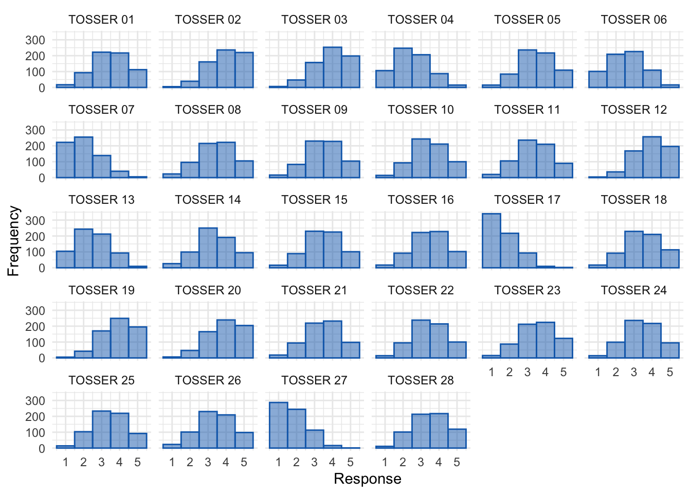
Distributions for items
tosr_tidy_tib <- tosr_items_tib %>%
  tidyr::pivot_longer(
    cols = tosr_01:tosr_28,
    names_to = "Item",
    values_to = "Response"
  ) %>%
  dplyr::mutate(
    Item = gsub("tosr_", "TOSSER ", Item)
  )

ggplot2::ggplot(tosr_tidy_tib, aes(Response)) +
  geom_histogram(binwidth = 1, fill = "#136CB9", colour = "#136CB9", alpha = 0.5) +
  labs(y = "Frequency") +
  facet_wrap(~ Item, ncol = 6) +
  theme_minimal()
Parallel analysis
psych::fa.parallel(tosr_cor, fm = "ml", fa = "fa", n.obs = 661)
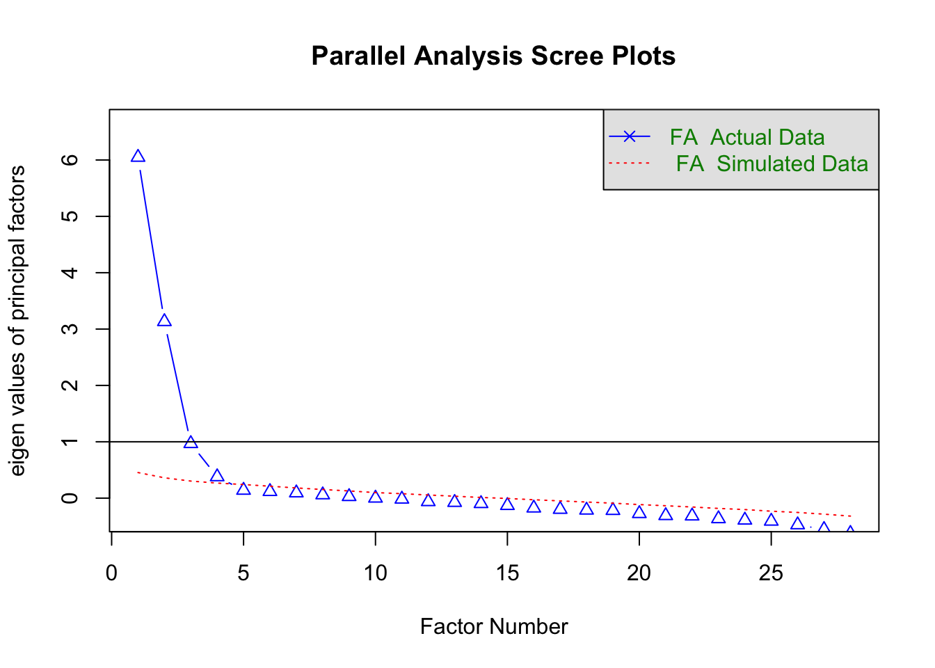
## Parallel analysis suggests that the number of factors = 4 and the number of components = NA
Based on parallel analysis five factors should be extracted.
Factor analysis
Create the factor analysis object. The question asks us to use maximum likelihood so I have included fm = "ml". We choose an oblique rotation (the default) because the question says that the constructs we’re measuring are related.
tosr_fa <- psych::fa(tosr_cor,
                    n.obs = 661,
                    fm = "ml",
                    nfactors = 4,
                    scores = "tenBerge"
                    )
summary(tosr_fa)
##
## Factor analysis with Call: psych::fa(r = tosr_cor, nfactors = 4, n.obs = 661, scores = "tenBerge",
##     fm = "ml")
##
## Test of the hypothesis that 4 factors are sufficient.
## The degrees of freedom for the model is 272  and the objective function was  0.7
## The number of observations was  661  with Chi Square =  450.06  with prob <  6.1e-11
##
## The root mean square of the residuals (RMSA) is  0.02
## The df corrected root mean square of the residuals is  0.03
##
## Tucker Lewis Index of factoring reliability =  0.959
## RMSEA index =  0.031  and the 10 % confidence intervals are  0.026 0.037
## BIC =  -1316.24
##  With factor correlations of
##       ML1  ML3  ML2   ML4
## ML1  1.00 0.08 0.11 -0.39
## ML3  0.08 1.00 0.32  0.23
## ML2  0.11 0.32 1.00  0.31
## ML4 -0.39 0.23 0.31  1.00
In terms of fit
- The chi-square statistic is $ \chi^2 = $(272) 450.06, p < 0.001. This is consistent with when we ran the analysis as factor analysis in the chapter.
- The Tucker Lewis Index of factoring reliability (TFI) is given as 0.96, which is equal to 0.96.
- The RMSEA = 0.031 90% CI [0.026, 0.037], which is below than 0.05.
- The RMSR is 0.02, which is smaller than both 0.09 and 0.06.
Remember that we’re looking for a combination of TLI > 0.96 and SRMR (RMSR in the output) < 0.06, and a combination of RMSEA < 0.05 and SRMR < 0.09. With the caveat that universal cut-offs need to be taken with a pinch of salt, it’s reasonable to conclude that the model has good fit.
Inspect the factor loadings:
parameters::model_parameters(tosr_fa, threshold = 0.2, sort = TRUE) %>%
  knitr::kable(digits = 2)
| Variable | ML1 | ML3 | ML2 | ML4 | Complexity | Uniqueness |
|---|---|---|---|---|---|---|
| tosr\_02 | -0.79 | 1.07 | 0.42 | |||
| tosr\_19 | 0.76 | 1.12 | 0.30 | |||
| tosr\_20 | 0.72 | 1.15 | 0.44 | |||
| tosr\_10 | 0.69 | 0.32 | 1.49 | 0.41 | ||
| tosr\_26 | 0.69 | 1.12 | 0.43 | |||
| tosr\_25 | 0.68 | 1.07 | 0.49 | |||
| tosr\_06 | -0.66 | 1.07 | 0.55 | |||
| tosr\_07 | 0.62 | 1.08 | 0.56 | |||
| tosr\_27 | -0.59 | 1.07 | 0.68 | |||
| tosr\_11 | 0.54 | 1.35 | 0.58 | |||
| tosr\_18 | 0.48 | 1.29 | 0.69 | |||
| tosr\_14 | 0.65 | 0.27 | 1.48 | 0.35 | ||
| tosr\_17 | 0.63 | 1.18 | 0.58 | |||
| tosr\_16 | 0.55 | 1.20 | 0.68 | |||
| tosr\_22 | 0.50 | 1.06 | 0.78 | |||
| tosr\_08 | 0.49 | -0.26 | 1.73 | 0.70 | ||
| tosr\_13 | 0.48 | 1.14 | 0.79 | |||
| tosr\_09 | 0.34 | 0.34 | 2.37 | 0.68 | ||
| tosr\_21 | 0.62 | 1.07 | 0.60 | |||
| tosr\_04 | 0.26 | 0.56 | 1.62 | 0.44 | ||
| tosr\_01 | 0.52 | 1.13 | 0.70 | |||
| tosr\_03 | 0.46 | 1.60 | 0.81 | |||
| tosr\_24 | 0.40 | 1.29 | 0.77 | |||
| tosr\_15 | 0.36 | 0.33 | 2.10 | 0.65 | ||
| tosr\_05 | 0.56 | 1.07 | 0.67 | |||
| tosr\_28 | -0.35 | 0.48 | 1.98 | 0.46 | ||
| tosr\_23 | -0.28 | 0.44 | 1.72 | 0.62 | ||
| tosr\_12 | -0.22 | 0.36 | 1.96 | 0.76 |
Factor 1
This factor seems to relate to teaching.
- Q2: I wish students would stop bugging me with their shit.
- Q19: I like to help students
- Q20: Passing on knowledge is the greatest gift you can bestow an individual
- Q10: I could spend all day explaining statistics to people
- Q26: I spend lots of time helping students
- Q25: I love teaching
- Q6: Teaching others makes me want to swallow a large bottle of bleach because the pain of my burning oesophagus would be light relief in comparison
- Q7: Helping others to understand sums of squares is a great feeling
- Q27: I love teaching because students have to pretend to like me or they’ll get bad marks
- Q11: I like it when people tell me I’ve helped them to understand factor rotation
- Q18: Standing in front of 300 people in no way makes me lose control of my bowels
Factor 2
This factor 1 seems to relate to research methods.
- Q14: I’d rather think about appropriate outcome variables than go for a drink with my friends
- Q17: I enjoy sitting in the park contemplating whether to use participant observation in my next experiment
- Q16: Thinking about whether to use repeated or independent measures thrills me
- Q22: I quiver with excitement when thinking about designing my next experiment
- Q8: I like control conditions
- Q13: Designing experiments is fun
- Q9: I calculate 3 ANOVAs in my head before getting out of bed [equally loaded on factor 3]
Factor 3
This factor seems to relate to statistics.
- Q9: I calculate 3 ANOVAs in my head before getting out of bed [equally loaded on factor 3]
- Q21: Thinking about Bonferroni corrections gives me a tingly feeling in my groin
- Q4: I worship at the shrine of Pearson
- Q1: I once woke up in the middle of a vegetable patch hugging a turnip that I’d mistakenly dug up thinking it was Roy’s largest root
- Q3: I memorize probability values for the F-distribution
- Q 24: I tried to build myself a time machine so that I could go back to the 1930s and follow Mahalanobis on my hands and knees licking the ground on which he’d just trodden
- Q15: I soil my pants with excitement at the mere mention of factor analysis [equally loaded on factor 4]
Factor 4
This factor seems to relate to social functioning. Not sure where the soiling pants comes in but probably if you’re the sort of person who soils their pants at the mention of factor analysis then things are going to get social awkward for you sooner rather than later.
- Q5: I still live with my mother and have little personal hygiene
- Q28: My cat is my only friend
- Q23: I often spend my spare time talking to the pigeons … and even they die of boredom
- Q12: People fall asleep as soon as I open my mouth to speak
- Q15: I soil my pants with excitement at the mere mention of factor analysis [equally loaded on factor 4]
Task 18.3
Dr Sian Williams (University of Brighton) devised a questionnaire to measure organizational ability. She predicted five components to do with organizational ability:(1) preference for organization; (2) goal achievement; (3) planning approach; (4) acceptance of delays; and (5) preference for routine. Williams’s questionnaire contains 28 items using a seven-point Likert scale (1 = strongly disagree, 4 = neither, 7 = strongly agree). She gave it to 239 people. Run a factor analysis (following the settings in this chapter) on the data in williams.csv.
Load the data
To load the data from the CSV file (assuming you have set up a project folder as suggested in the book):
org_tib <- here::here("data/williams.csv") %>%
  readr::read_csv()
Alternative, load the data directly from the discovr package:
org_tib <- discovr::williams
Fit the model
The questionnaire items are as follows:
- I like to have a plan to work to in everyday life
- I feel frustrated when things don’t go to plan
- I get most things done in a day that I want to
- I stick to a plan once I have made it
- I enjoy spontaneity and uncertainty
- I feel frustrated if I can’t find something I need
- I find it difficult to follow a plan through
- I am an organized person
- I like to know what I have to do in a day
- Disorganized people annoy me
- I leave things to the last minute
- I have many different plans relating to the same goal
- I like to have my documents filed and in order
- I find it easy to work in a disorganized environment
- I make ‘to do’ lists and achieve most of the things on it
- My workspace is messy and disorganized
- I like to be organized
- Interruptions to my daily routine annoy me
- I feel that I am wasting my time
- I forget the plans I have made
- I prioritize the things I have to do
- I like to work in an organized environment
- I feel relaxed when I don’t have a routine
- I set deadlines for myself and achieve them
- I change rather aimlessly from one activity to another during the day
- I have trouble organizing the things I have to do
- I put tasks off to another day
- I feel restricted by schedules and plans
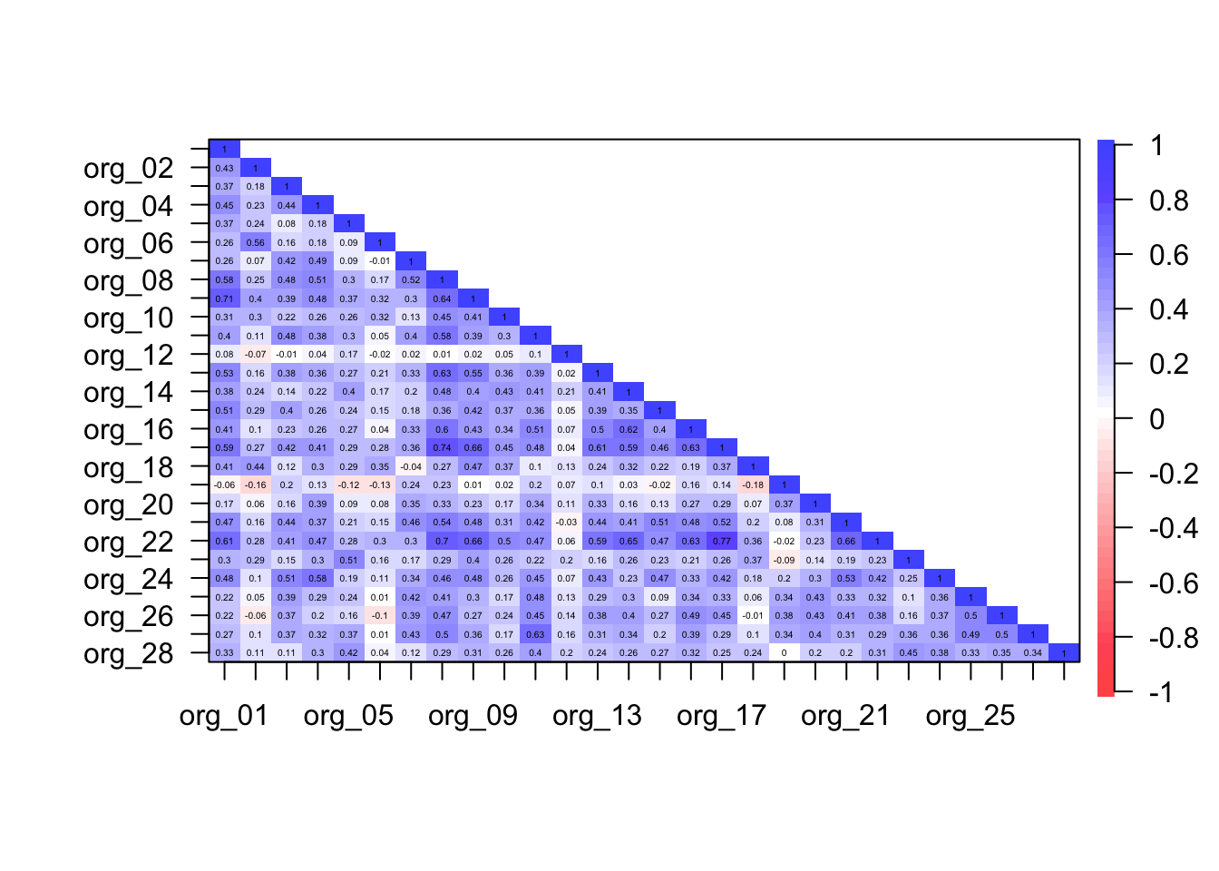
Create correlation matrix
The data file has a variables in it containing participants’ demographic information. Let’s store a version of the data that only has the item scores.
org_items_tib <- org_tib %>%
  dplyr::select(-id)
We can create the correlations between variables by executing (again, items were rated on Likert response scales, so we’ll use polychoric correlations).
org_poly <- psych::polychoric(org_items_tib)
org_cor <- org_poly$rho
To get a plot of the correlations we can execute:
psych::cor.plot(org_cor, upper = FALSE)
The Bartlett test
psych::cortest.bartlett(org_cor, n = 239)
## $chisq
## [1] 3679.19
##
## $p.value
## [1] 0
##
## $df
## [1] 378
This (basically useless) tests confirms that the correlation matrix is significantly different from an identity matrix (i.e. correlations are non-zero).
Determinant of the correlation matrix:
det(org_cor)
## [1] 9.699541e-08
The determinant of the correlation matrix was 0.00000009699541, which is smaller than 0.00001 and, therefore, indicates that multicollinearity could be a problem in these data.
The KMO test
psych::KMO(org_cor)
## Kaiser-Meyer-Olkin factor adequacy
## Call: psych::KMO(r = org_cor)
## Overall MSA =  0.88
## MSA for each item =
## org_01 org_02 org_03 org_04 org_05 org_06 org_07 org_08 org_09 org_10 org_11
##   0.93   0.78   0.84   0.82   0.85   0.76   0.83   0.94   0.94   0.90   0.91
## org_12 org_13 org_14 org_15 org_16 org_17 org_18 org_19 org_20 org_21 org_22
##   0.57   0.93   0.88   0.88   0.94   0.91   0.85   0.76   0.79   0.85   0.88
## org_23 org_24 org_25 org_26 org_27 org_28
##   0.82   0.89   0.87   0.90   0.86   0.82
The KMO measure of sampling adequacy is 0.88, which is above Kaiser’s (1974) recommendation of 0.5. This value is also ‘meritorious’ (and almost ‘marvellous’). Individual items KMO values ranged from 0.57 to 0.94. As such, the evidence suggests that the sample size is adequate to yield distinct and reliable factors.
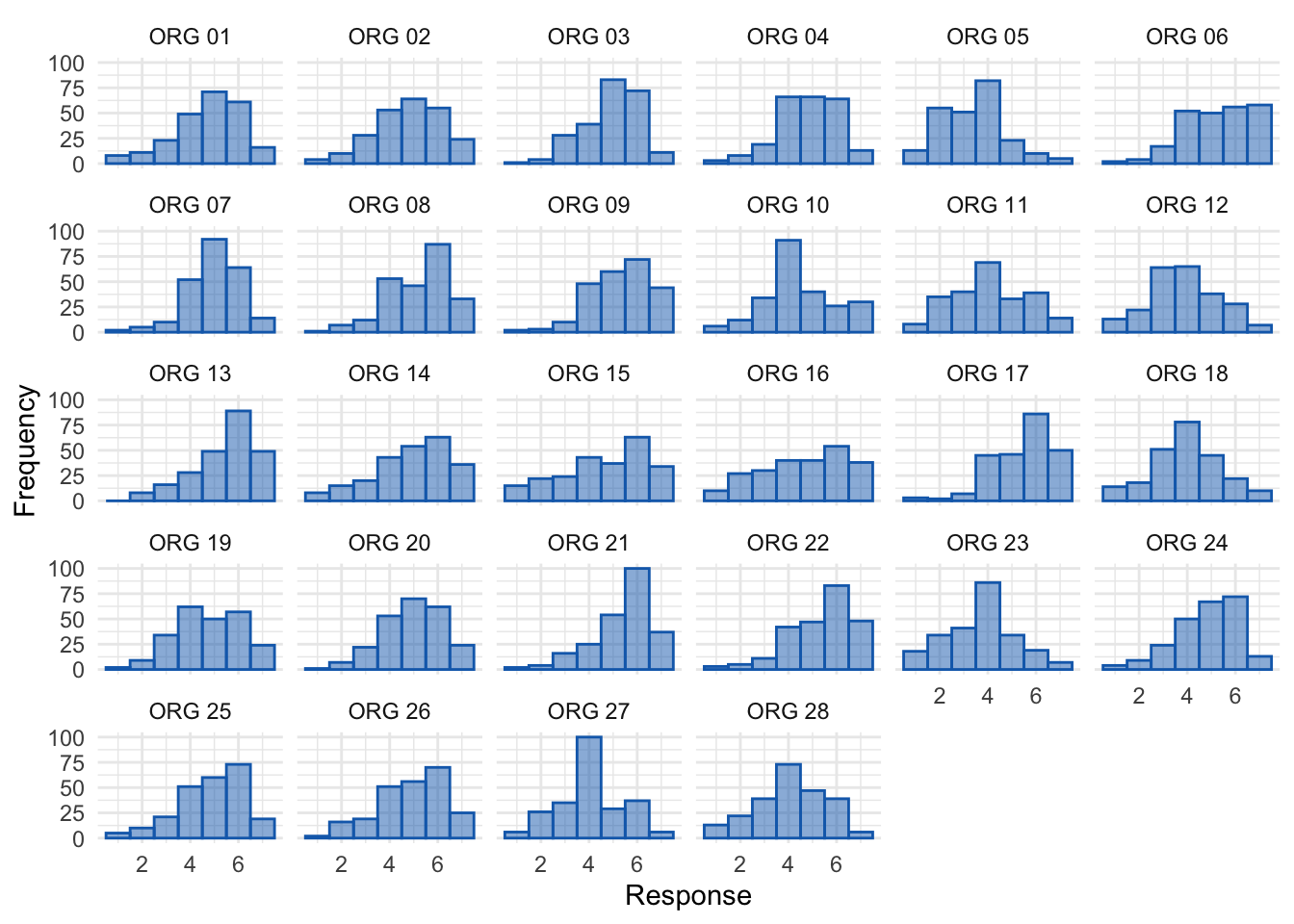
Distributions for items
org_tidy_tib <- org_items_tib %>%
  tidyr::pivot_longer(
    cols = org_01:org_28,
    names_to = "Item",
    values_to = "Response"
  ) %>%
  dplyr::mutate(
    Item = gsub("org_", "ORG ", Item)
  )

ggplot2::ggplot(org_tidy_tib, aes(Response)) +
  geom_histogram(binwidth = 1, fill = "#136CB9", colour = "#136CB9", alpha = 0.5) +
  labs(y = "Frequency") +
  facet_wrap(~ Item, ncol = 6) +
  theme_minimal()
Parallel analysis
psych::fa.parallel(org_cor, fm = "ml", fa = "fa", n.obs = 239)
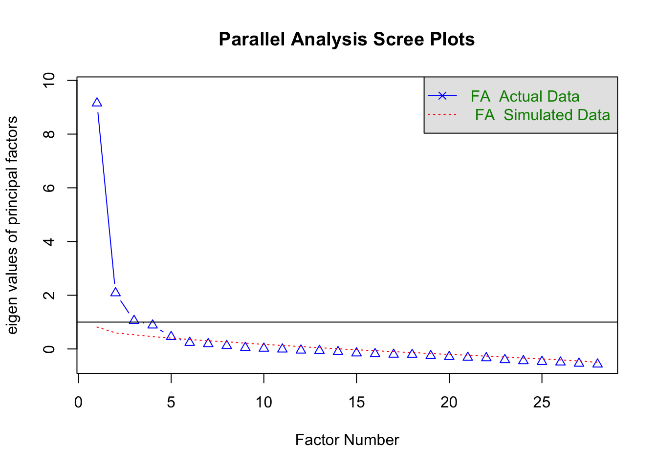
## Parallel analysis suggests that the number of factors = 5 and the number of components = NA
Based on parallel analysis five factors should be extracted.
Factor analysis
Create the factor analysis object. The question asks us to use maximum likelihood so I have included fm = "ml". We choose an oblique rotation (the default) because the question says that the constructs we’re measuring are related.
org_fa <- psych::fa(org_cor,
                    n.obs = 239,
                    fm = "minres",
                    nfactors = 5
                    )
summary(org_fa)
##
## Factor analysis with Call: psych::fa(r = org_cor, nfactors = 5, n.obs = 239, fm = "minres")
##
## Test of the hypothesis that 5 factors are sufficient.
## The degrees of freedom for the model is 248  and the objective function was  2.51
## The number of observations was  239  with Chi Square =  563.4  with prob <  1.4e-26
##
## The root mean square of the residuals (RMSA) is  0.04
## The df corrected root mean square of the residuals is  0.04
##
## Tucker Lewis Index of factoring reliability =  0.852
## RMSEA index =  0.073  and the 10 % confidence intervals are  0.065 0.081
## BIC =  -794.77
##  With factor correlations of
##      MR1   MR2  MR4  MR3   MR5
## MR1 1.00  0.35 0.45 0.38  0.30
## MR2 0.35  1.00 0.35 0.21 -0.08
## MR4 0.45  0.35 1.00 0.22  0.29
## MR3 0.38  0.21 0.22 1.00  0.25
## MR5 0.30 -0.08 0.29 0.25  1.00
In terms of fit
- The chi-square statistic is $ \chi^2 = $(248) 563.4, p < 0.001. This is consistent with when we ran the analysis as factor analysis in the chapter.
- The Tucker Lewis Index of factoring reliability (TFI) is given as 0.85, which is well below 0.96.
- The RMSEA = 0.073 90% CI [0.065, 0.081], which is greater than 0.05.
- The RMSR is 0.04, which is smaller than both 0.09 and 0.06.
Remember that we’re looking for a combination of TLI > 0.96 and SRMR (RMSR in the output) < 0.06, and a combination of RMSEA < 0.05 and SRMR < 0.09. With the caveat that universal cut-offs need to be taken with a pinch of salt, it’s reasonable to conclude that the model has poor fit.
Inspect the factor loadings:
parameters::model_parameters(org_fa, threshold = 0.2, sort = TRUE) %>%
  knitr::kable(digits = 2)
| Variable | MR1 | MR2 | MR4 | MR3 | MR5 | Complexity | Uniqueness |
|---|---|---|---|---|---|---|---|
| org\_14 | 0.78 | -0.27 | 1.38 | 0.34 | |||
| org\_16 | 0.78 | 1.14 | 0.35 | ||||
| org\_22 | 0.77 | 0.20 | 1.22 | 0.19 | |||
| org\_17 | 0.72 | 1.25 | 0.25 | ||||
| org\_08 | 0.50 | 0.30 | 0.22 | 2.31 | 0.28 | ||
| org\_13 | 0.49 | 0.24 | 1.62 | 0.51 | |||
| org\_10 | 0.40 | 0.27 | 1.94 | 0.65 | |||
| org\_19 | 0.63 | 1.23 | 0.60 | ||||
| org\_27 | 0.61 | 0.34 | 1.58 | 0.39 | |||
| org\_25 | 0.60 | 1.12 | 0.52 | ||||
| org\_20 | 0.58 | 1.09 | 0.63 | ||||
| org\_26 | 0.38 | 0.47 | -0.25 | 2.56 | 0.42 | ||
| org\_07 | 0.46 | 0.32 | 1.90 | 0.57 | |||
| org\_11 | 0.26 | 0.36 | 0.21 | 0.20 | 3.30 | 0.47 | |
| org\_24 | 0.69 | 1.22 | 0.39 | ||||
| org\_03 | 0.25 | 0.55 | 1.55 | 0.51 | |||
| org\_04 | 0.26 | 0.49 | 0.24 | 2.21 | 0.49 | ||
| org\_21 | 0.43 | 0.45 | 2.05 | 0.46 | |||
| org\_15 | 0.36 | -0.22 | 0.44 | 2.72 | 0.56 | ||
| org\_01 | 0.31 | 0.43 | 0.22 | 3.11 | 0.38 | ||
| org\_23 | 0.66 | 1.25 | 0.49 | ||||
| org\_05 | 0.65 | 1.10 | 0.51 | ||||
| org\_28 | 0.63 | 1.18 | 0.53 | ||||
| org\_12 | 0.33 | 1.70 | 0.87 | ||||
| org\_02 | 0.71 | 1.04 | 0.45 | ||||
| org\_06 | 0.70 | 1.06 | 0.53 | ||||
| org\_18 | 0.28 | 0.47 | 2.04 | 0.55 | |||
| org\_09 | 0.32 | 0.32 | 0.34 | 3.46 | 0.34 |
Factor 1
This factor 1 seems to relate to preference for organization.
- Q14: I find it easy to work in a disorganized environment
- Q16: My workspace is messy and disorganized
- Q22: I like to work in an organized environment
- Q17: I like to be organized
- Q8: I am an organized person
- Q13: I like to have my documents filed and in order
- Q10: Disorganized people annoy me
Factor 2
This factor seems to relate to goal achievement (it probably depends how you define goal achievement but does seem to relate to your ability to follow a plan through!).
- Q19: I feel that I am wasting my time
- Q27: I put tasks off to another day
- Q25: I change rather aimlessly from one activity to another during the day
- Q20: I forget the plans I have made
- Q26: I have trouble organizing the things I have to do
- Q7: I find it difficult to follow a plan through
- Q11: I leave things to the last minute
Factor 3
This factor seems to relate to planning approach.
- Q24: I set deadlines for myself and achieve them
- Q3: I get most things done in a day that I want to
- Q4: I stick to a plan once I have made it
- Q21: I prioritize the things I have to do
- Q15: I make ‘to do’ lists and achieve most of the things on it
- Q1: I like to have a plan to work to in everyday life
Factor 4
This factor seems to relate to preference for routine.
- Q23: I feel relaxed when I don’t have a routine
- Q5: I enjoy spontaneity and uncertainty
- Q28: I feel restricted by schedules and plans
- Q12: I have many different plans relating to the same goal
Factor 5
This factor seems to relate to acceptance of delays.
- Q2: I feel frustrated when things don’t go to plan
- Q6: I feel frustrated if I can’t find something I need
- Q18: Interruptions to my daily routine annoy me
- Q9: I like to know what I have to do in a day
It seems as though there is some factorial validity to the hypothesized structure. (But remember that this model has poor fit.)
Task 18.4
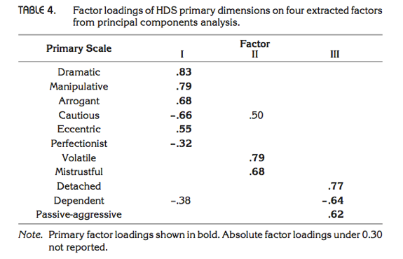
Zibarras et al., (2008) looked at the relationship between personality and creativity. They used the Hogan Development Survey (HDS), which measures 11 dysfunctional dispositions of employed adults: being volatile, mistrustful, cautious, detached, passive_aggressive, arrogant, manipulative, dramatic, eccentric, perfectionist, and dependent. Zibarras et al. wanted to reduce these 11 traits down and, based on parallel analysis, found that they could be reduced to three components. They ran a principal component analysis with varimax rotation. Repeat this analysis (zibarras_2008.csv) to see which personality dimensions clustered together (see page 210 of the original paper).
Load the data
To load the data from the CSV file (assuming you have set up a project folder as suggested in the book):
zibarras_tib <- here::here("data/zibarras_2018.csv") %>%
  readr::read_csv()
Alternative, load the data directly from the discovr package:
zibarras_tib <- discovr::zibarras_2008
Like the authors, I ran the analysis with principal components and varimax rotation.
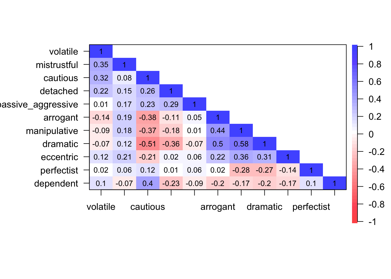
Create correlation matrix
The data file has a variable in it containing participants’ ids. Let’s store a version of the data that only has the item scores.
zibarras_tib <- zibarras_tib %>%
  dplyr::select(-id)
We can create the correlations between variables by executing.
zibarras_cor <- cor(zibarras_tib)
To get a plot of the correlations we can execute:
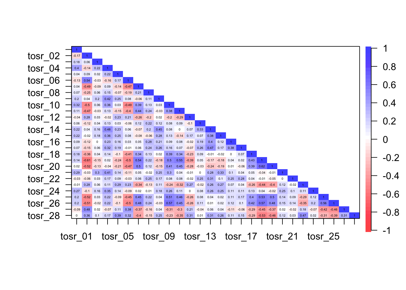
psych::cor.plot(zibarras_cor, upper = FALSE)
The Bartlett test
psych::cortest.bartlett(zibarras_cor, n = 207)
## $chisq
## [1] 527.8976
##
## $p.value
## [1] 1.841689e-78
##
## $df
## [1] 55
This (basically useless) tests confirms that the correlation matrix is significantly different from an identity matrix (i.e. correlations are non-zero).
The KMO test
psych::KMO(zibarras_cor)
## Kaiser-Meyer-Olkin factor adequacy
## Call: psych::KMO(r = zibarras_cor)
## Overall MSA =  0.68
## MSA for each item =
##           volatile        mistrustful           cautious           detached
##               0.52               0.62               0.71               0.56
## passive_aggressive           arrogant       manipulative           dramatic
##               0.50               0.76               0.81               0.72
##          eccentric         perfectist          dependent
##               0.82               0.54               0.58
The KMO measure of sampling adequacy is 0.68, which is above Kaiser’s (1974) recommendation of 0.5. Individual items KMO values ranged from 0.5 to 0.82. Thee values are in the mediocre to middling range. The sample size is probably adequate to yield distinct and reliable factors.
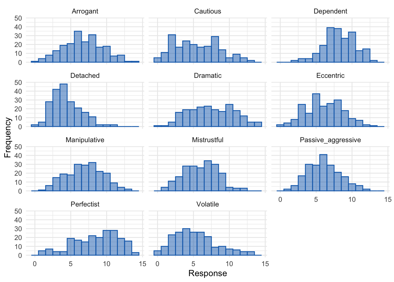
Distributions for items
zib_tidy_tib <- zibarras_tib %>%
  tidyr::pivot_longer(
    cols = volatile:dependent,
    names_to = "Item",
    values_to = "Response"
  ) %>%
  dplyr::mutate(
    Item = stringr::str_to_sentence(Item)
  )

ggplot2::ggplot(zib_tidy_tib, aes(Response)) +
  geom_histogram(binwidth = 1, fill = "#136CB9", colour = "#136CB9", alpha = 0.5) +
  labs(y = "Frequency") +
  facet_wrap(~ Item, ncol = 3) +
  theme_minimal()
Parallel analysis
psych::fa.parallel(zibarras_cor, fa = "pc", n.obs = 207)
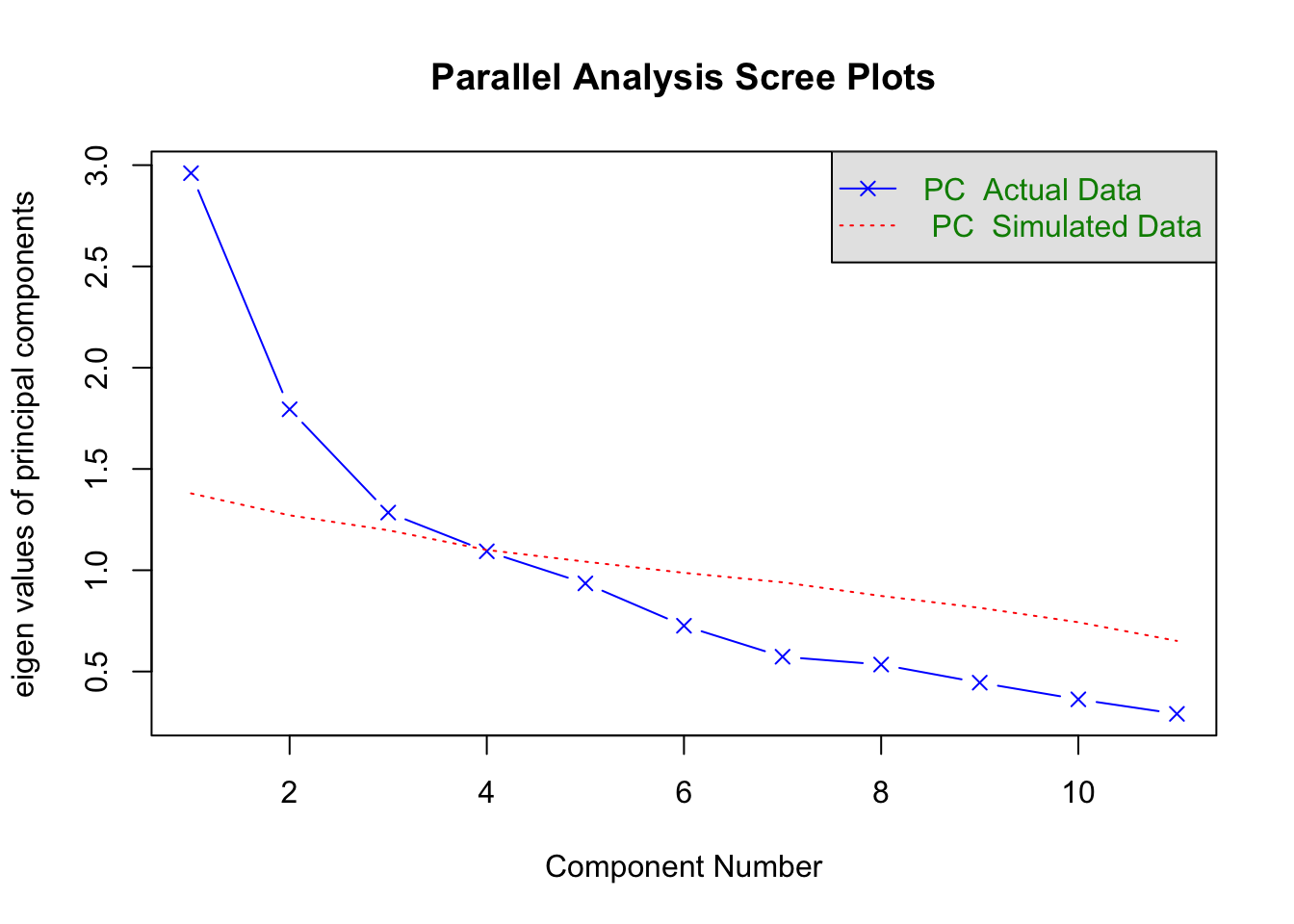
## Parallel analysis suggests that the number of factors = NA and the number of components = 3
Based on parallel analysis three components should be extracted (as the authors did in the paper).
PCA
Create the PCA object. We choose an orthogonal rotation (varimax) because that’s what the authors did - this is the default for PCA so we don’t need to specify it explicitly.
zib_pca <- psych::pca(zibarras_cor,
                    n.obs = 207,
                    nfactors = 3
                    )
summary(zib_pca)
##
## Factor analysis with Call: principal(r = r, nfactors = nfactors, residuals = residuals,
##     rotate = rotate, n.obs = n.obs, covar = covar, scores = scores,
##     missing = missing, impute = impute, oblique.scores = oblique.scores,
##     method = method, use = use, cor = cor, correct = 0.5, weight = NULL)
##
## Test of the hypothesis that 3 factors are sufficient.
## The degrees of freedom for the model is 25  and the objective function was  0.92
## The number of observations was  207  with Chi Square =  182.93  with prob <  5.7e-26
##
## The root mean square of the residuals (RMSA) is  0.1
Inspect the factor loadings:
parameters::model_parameters(zib_pca, threshold = 0.2, sort = TRUE) %>%
  knitr::kable(digits = 2)
| Variable | RC1 | RC2 | RC3 | Complexity | Uniqueness |
|---|---|---|---|---|---|
| dramatic | 0.83 | 1.11 | 0.27 | ||
| manipulative | 0.79 | 1.03 | 0.37 | ||
| arrogant | 0.68 | 1.06 | 0.53 | ||
| cautious | -0.66 | 0.50 | 1.87 | 0.31 | |
| eccentric | 0.55 | 0.30 | 1.73 | 0.59 | |
| perfectist | -0.32 | 1.09 | 0.89 | ||
| volatile | 0.79 | 1.03 | 0.37 | ||
| mistrustful | 0.27 | 0.68 | 0.24 | 1.58 | 0.40 |
| detached | -0.28 | 0.76 | 1.39 | 0.30 | |
| dependent | -0.38 | 0.33 | -0.64 | 2.21 | 0.33 |
| passive\_aggressive | 0.62 | 1.17 | 0.59 |
The output shows the rotated component matrix, from which we see this pattern:
- Component 1:
- Dramatic
- Manipulative
- Arrogant
- Cautious (negative weight)
- Eccentric
- Perfectionist (negative weight)
- Component 2:
- Volatile
- Mistrustful
- Component 3:
- Detached
- Dependent (negative weight)
- Passive-aggressive
Compare these results to those of Zibarras et al. (Table 4 from the original paper reproduced below), and note that they are the same.