Smart Alex solutions Chapter 13
Task 13.1
People have claimed that listening to heavy metal, because of its aggressive sonic palette and often violent or emotionally negative lyrics, leads to angry and aggressive behaviour (Selfhout et al., 2008). As a very non-violent metal fan this accusation bugs me. Imagine I designed a study to test this possibility. I took groups of self-classifying metalheads and non-metalheads (fan) and assigned them randomly to listen to 15 minutes of either the sound of an angle grinder scraping a sheet of metal (control noise), metal music, or pop music (soundtrack). Each person rated their anger on a scale ranging from 0 (“All you need is love, da, da, da-da-da”) to 100 (“Fuck me, I’m all out of enemies”). Fit a model to test my idea (metal.csv).
Load the data
To load the data from the CSV file (assuming you have set up a project folder as suggested in the book) and set the factor and its levels:
metal_tib <- readr::read_csv("../data/metal.csv") %>%
  dplyr::mutate(
    soundtrack = forcats::as_factor(soundtrack) %>% forcats::fct_relevel(., "Angle grinder"),
    fan = forcats::as_factor(fan)
  )
Alternative, load the data directly from the discovr package:
metal_tib <- discovr::metal
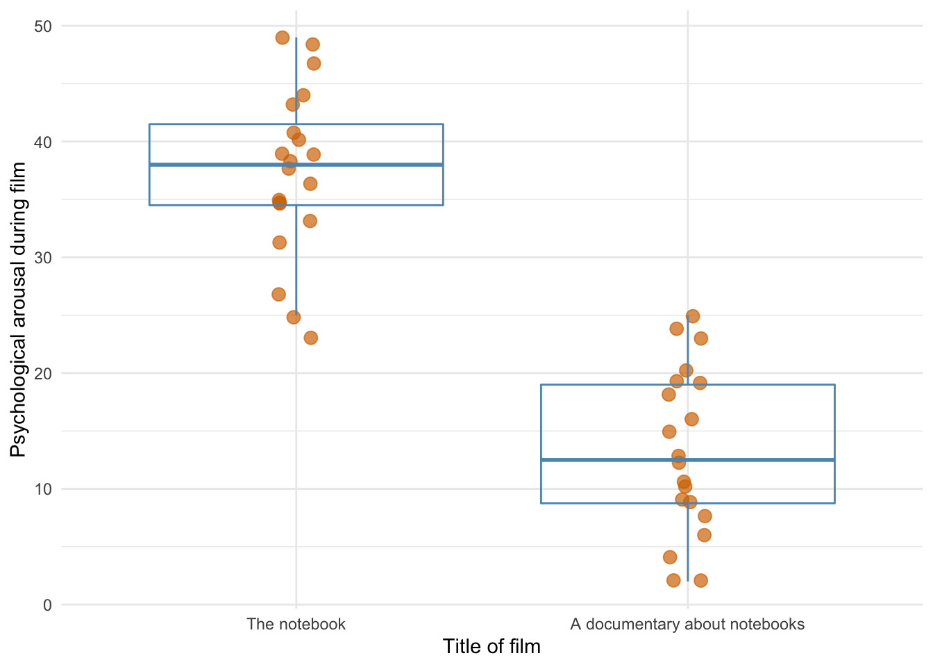
Plot the data
ggplot2::ggplot(metal_tib, aes(x = soundtrack, y = anger, colour = fan)) +
  geom_violin(alpha = 0.5) +
  stat_summary(fun.data = "mean_cl_normal", position = position_dodge(width = 0.9)) +
  scale_y_continuous(breaks = seq(0, 100, 10)) +
  labs(y = "Anger (out of 100)", x = "Soundtrack", colour = "Fan group") +
  discovr::scale_colour_pom() +
  theme_minimal()
The plot shows that after listening to an angle grinder both groups are angry. After listening to metal, the metal heads score low on anger but the pop fans score high. the reverse is true after listening to pop music.
Fitting the model using afex::aov_4()
metal_afx <- afex::aov_4(anger ~ soundtrack*fan + (1|id), data = metal_tib)
metal_afx
## Anova Table (Type 3 tests)
##
## Response: anger
##           Effect    df   MSE          F   ges p.value
## 1     soundtrack 2, 84 87.61 116.82 ***  .736   <.001
## 2            fan 1, 84 87.61       0.07 <.001    .788
## 3 soundtrack:fan 2, 84 87.61 433.28 ***  .912   <.001
## ---
## Signif. codes:  0 '***' 0.001 '**' 0.01 '*' 0.05 '+' 0.1 ' ' 1
Fitting the model using lm()
Set contrasts for fan:
metal_vs_pop <- c(-0.5, 0.5)
contrasts(metal_tib$fan) <- metal_vs_pop
Set contrasts for soundtrack. What we really want here is a contrast that compares metal against pop and the angle grinder, but this contrast isn’t orthogonal and we need orthogonal contrasts for the type III sums of squares. Instead we’ll use the build in contr.sum, which will give us ‘sum to zero’ contrasts, which are orthogonal.
contrasts(metal_tib$soundtrack) <- contr.sum(3)
Fit the model and print Type III sums of squares:
metal_lm <- lm(anger ~ soundtrack*fan, data = metal_tib)
car::Anova(metal_lm, type = 3)
## Anova Table (Type III tests)
##
## Response: anger
##                Sum Sq Df   F value Pr(>F)
## (Intercept)    321365  1 3668.1557 <2e-16 ***
## soundtrack      20470  2  116.8238 <2e-16 ***
## fan                 6  1    0.0731 0.7876
## soundtrack:fan  75919  2  433.2820 <2e-16 ***
## Residuals        7359 84
## ---
## Signif. codes:  0 '***' 0.001 '**' 0.01 '*' 0.05 '.' 0.1 ' ' 1
Interpret the mode
The resulting output can be interpreted as follows.
- The main effect of soundtrack was significant, F(2, 84) = 116.82, p < .001, indicating that anger scores were significantly different across the three soundtracks. From the EMMs below it seems that after listening to the angle grinder anger was higher than after both both pop and metal (but if we cared about this main effect we’d need to test this formally).
emmeans::emmeans(metal_afx, "soundtrack")
##  soundtrack    emmean   SE df lower.CL upper.CL
##  Angle grinder   81.0 1.71 84     77.6     84.4
##  Metal           47.5 1.71 84     44.1     50.9
##  Pop             50.8 1.71 84     47.4     54.2
##
## Results are averaged over the levels of: fan
## Confidence level used: 0.95
- The main effect of fan was not significant, F(1, 84) = 0.07, p = 0.788, indicating that anger scores were not significantly different overall between metal and pop fans.
- The soundtrack × fan interaction was significant, F(2, 84) = 433.28, p < .001, indicating that the soundtrack combined with the type of fan significantly affected anger. The plot shows that after listening to an angle grinder both groups are angry. After listening to metal, the metal heads score low on anger but the pop fans score high. the reverse is true after listening to pop music. We can test this formally with simple effects analysis.
emmeans::joint_tests(metal_afx, "soundtrack")
## soundtrack = Angle grinder:
##  model term df1 df2 F.ratio p.value
##  fan          1  84   0.298 0.5864
##
## soundtrack = Metal:
##  model term df1 df2 F.ratio p.value
##  fan          1  84 431.546 <.0001
##
## soundtrack = Pop:
##  model term df1 df2 F.ratio p.value
##  fan          1  84 434.793 <.0001
Yes, it looks like metal and pop fans do not significantly differ in anger after listening to an angle grinder, but metal; fans have significantly greater anger after listening to pop and vice versa for the pop fans.
Task 13.2
Compute omega squared for the effects in Task 1 and report the results of the analysis.
Omega squared for models using aov_4() (for the model using lm() replace metal_afx with metal_lm)
effectsize::omega_squared(metal_afx, ci = 0.95, partial = FALSE)
## # Effect Size for ANOVA (Type III)
##
## Parameter      |    Omega2 |       95% CI
## -----------------------------------------
## soundtrack     |      0.20 | [0.06, 0.33]
## fan            | -7.82e-04 | [0.00, 0.00]
## soundtrack:fan |      0.73 | [0.63, 0.79]
We could report (remember if you’re using APA format to drop the leading zeros before p-values and ω2, for example report p = .035 instead of p = 0.035):
- The main effect of soundtrack was significant, F(2, 84) = 116.82, p < .001, ω2 = 0.2, 95% CI [0.06, 0.33] indicating that anger scores were significantly different across the three soundtracks. It seems that after listening to the angle grinder anger was higher than after both both pop and metal.
- The main effect of fan was not significant, F(1, 84) = 0.07, p = 0.788, ω2 = 0, 95% CI [0, 0] indicating that anger scores were not significantly different overall between metal and pop fans. The effect was basically zero.
- The soundtrack × fan interaction was significant, F(2, 84) = 433.28, p < .001, ω2 = 0.73, 95% CI [0.63, 0.79] indicating that the soundtrack combined with the type of fan significantly affected anger. The plot shows that after listening to an angle grinder both groups are angry. After listening to metal, the metal heads score low on anger but the pop fans score high. the reverse is true after listening to pop music. This effect explained 73% of variance.
Task 13.3
In Chapter 5 we used some data that related to male and female arousal levels when watching The Notebook or a documentary about notebooks (notebook.csv). Fit a model to test whether men and women differ in their reactions to different types of films.
Load the data
To load the data from the CSV file (assuming you have set up a project folder as suggested in the book) and set the factor and its levels:
notebook_tib <- readr::read_csv("../data/notebook.csv") %>%
  dplyr::mutate(
    sex = forcats::as_factor(sex),
    film = forcats::as_factor(film),
  )
Load the data directly from the discovr package:
notebook_tib <- discovr::notebook
Fitting the model using aov_4()
notebook_afx <- afex::aov_4(arousal ~ film*sex + (1|id), data = notebook_tib)
notebook_afx
## Anova Table (Type 3 tests)
##
## Response: arousal
##     Effect    df   MSE          F  ges p.value
## 1     film 1, 36 40.77 141.87 *** .798   <.001
## 2      sex 1, 36 40.77     7.29 * .168    .011
## 3 film:sex 1, 36 40.77     4.64 * .114    .038
## ---
## Signif. codes:  0 '***' 0.001 '**' 0.01 '*' 0.05 '+' 0.1 ' ' 1
Fitting the model using lm()
Both sex and film have only two levels, so we don’t need contrasts to test hypothesises, but we need orthogonal ones for our Type III sums of squares. Let’s use the built in contr.sum to set these.
Set contrasts:
contrasts(notebook_tib$sex) <- contr.sum(2)
contrasts(notebook_tib$film) <- contr.sum(2)
Fit the model and print Type III sums of squares:
notebook_lm <- lm(arousal ~ film*sex, data = notebook_tib)
car::Anova(notebook_lm, type = 3)
## Anova Table (Type III tests)
##
## Response: arousal
##              Sum Sq Df  F value    Pr(>F)
## (Intercept) 25553.0  1 626.7690 < 2.2e-16 ***
## film         5784.0  1 141.8716  4.77e-14 ***
## sex           297.0  1   7.2855   0.01052 *
## film:sex      189.2  1   4.6413   0.03798 *
## Residuals    1467.7 36
## ---
## Signif. codes:  0 '***' 0.001 '**' 0.01 '*' 0.05 '.' 0.1 ' ' 1
Interpret the mode
The output shows that the main effect of sex is significant, F(1, 36) = 7.29, p = 0.011, as is the main effect of film, F(1, 36) = 141.87, p < .001 and the interaction, F(1, 36) = 4.64, p = 0.038. Let’s look at these effects in turn.
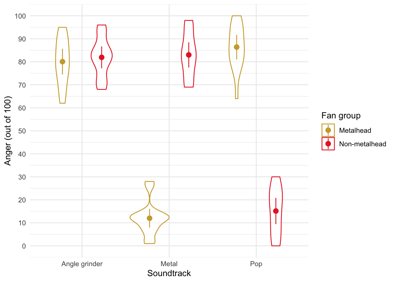
The graph of the main effect of sex shows that the significant effect is likely to reflect the fact that males experienced higher levels of psychological arousal in general than women (when the type of film is ignored).
ggplot(notebook_tib, aes(sex, arousal)) +
  geom_point(size = 3, position = position_jitter(width = 0.05), colour = ong, alpha = 0.7) +
  geom_boxplot(alpha = 0, colour = blu) +
  labs(x = "Biological sex", y = "Psychological arousal during film") +
  theme_minimal()
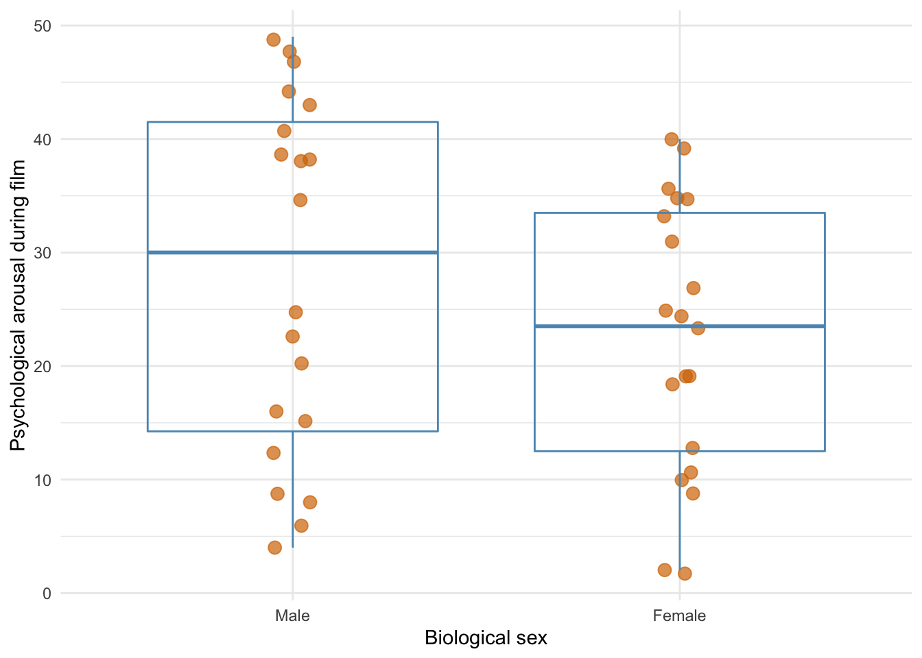
The main effect of the film was also significant, and the graph shows that when you ignore the biological sex of the participant, psychological arousal was higher during the notebook than during a documentary about notebooks.
ggplot(notebook_tib, aes(film, arousal)) +
  geom_point(size = 3, position = position_jitter(width = 0.05), colour = ong, alpha = 0.7) +
  geom_boxplot(alpha = 0, colour = blu) +
  labs(x = "Title of film", y = "Psychological arousal during film") +
  theme_minimal()
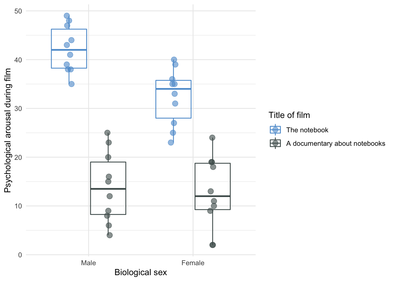
The interaction effect is shown in the plot of the data split by type of film and sex of the participant. Psychological arousal is very similar for men and women during the documentary about notebooks (it is low for both sexes). However, for the notebook men experienced greater psychological arousal than women. The interaction is likely to reflect that there is a difference between men and women for one type of film (the notebook) but not the other (the documentary about notebooks).
ggplot(notebook_tib, aes(sex, arousal, colour = film)) +
  geom_point(position = position_jitterdodge(dodge.width = 0.75, jitter.width = 0.1), size = 3, alpha = 0.6) +
  geom_boxplot(alpha = 0) +
  labs(x = "Biological sex", y = "Psychological arousal during film", colour = "Title of film") +
  discovr::scale_color_ssoass() +
  theme_minimal()
Task 13.4
Compute omega squared for the effects in Task 3 and report the results of the analysis.
Omega squared for models using aov_4() (for the model using lm() replace notebook_afx with notebook_lm)
effectsize::omega_squared(notebook_afx, ci = 0.95, partial = FALSE)
## # Effect Size for ANOVA (Type III)
##
## Parameter | Omega2 |       95% CI
## ---------------------------------
## film      |   0.74 | [0.58, 0.83]
## sex       |   0.03 | [0.00, 0.21]
## film:sex  |   0.02 | [0.00, 0.18]
We could report (remember if you’re using APA format to drop the leading zeros before p-values and ω2, for example report p = .035 instead of p = 0.035):
The results show that the psychological arousal during the films was significantly higher for males than females, F(1, 36) = 7.29, p = 0.011, ω2 = 0.03, 95% CI [0, 0.21]. Psychological arousal was also significantly higher during the notebook than during a documentary about notebooks, F(1, 36) = 141.87, p < .001, ω2 = 0.74, 95% CI [0.58, 0.83]. The interaction was also significant, F(1, 36) = 4.64, p = 0.038, ω2 = 0.02, 95% CI [0, 0.18], and seemed to reflect the fact that psychological arousal was very similar for men and women during the documentary about notebooks (it was low for both sexes), but for the notebook men experienced greater psychological arousal than women. However, the effect size for the interaction was trivial.
Task 13.5
In Chapter X we used some data that related to learning in men and women when either reinforcement or punishment was used in teaching (teach_method.csv). Analyse these data to see whether men and women’s learning differs according to the teaching method used.
Load the data
To load the data from the CSV file (assuming you have set up a project folder as suggested in the book) and set the factor and its levels:
teach_tib <- readr::read_csv("../data/teaching.csv") %>%
   dplyr::mutate(
    method = forcats::as_factor(method),
    sex = forcats::as_factor(sex)
  )
Load the data directly from the discovr package:
teach_tib <- discovr::teaching
Fitting the model using aov_4()
teach_afx <- afex::aov_4(mark ~ method*sex + (1|id), data = teach_tib)
teach_afx
## Anova Table (Type 3 tests)
##
## Response: mark
##       Effect    df  MSE         F  ges p.value
## 1     method 1, 16 5.00      2.25 .123    .153
## 2        sex 1, 16 5.00  12.25 ** .434    .003
## 3 method:sex 1, 16 5.00 30.25 *** .654   <.001
## ---
## Signif. codes:  0 '***' 0.001 '**' 0.01 '*' 0.05 '+' 0.1 ' ' 1
Fitting the model using lm()
Both sex and method have only two levels, so we don’t need contrasts to test hypothesises, but we need orthogonal ones for our Type III sums of squares. Let’s use the built in contr.sum to set these.
Set contrasts:
contrasts(teach_tib$sex) <- contr.sum(2)
contrasts(teach_tib$method) <- contr.sum(2)
Fit the model and print Type III sums of squares:
teach_lm <- lm(mark ~ method*sex, data = teach_tib)
car::Anova(teach_lm, type = 3)
## Anova Table (Type III tests)
##
## Response: mark
##              Sum Sq Df F value    Pr(>F)
## (Intercept) 1901.25  1  380.25 1.413e-12 ***
## method        11.25  1    2.25  0.153088
## sex           61.25  1   12.25  0.002964 **
## method:sex   151.25  1   30.25 4.845e-05 ***
## Residuals     80.00 16
## ---
## Signif. codes:  0 '***' 0.001 '**' 0.01 '*' 0.05 '.' 0.1 ' ' 1
Interpret the mode
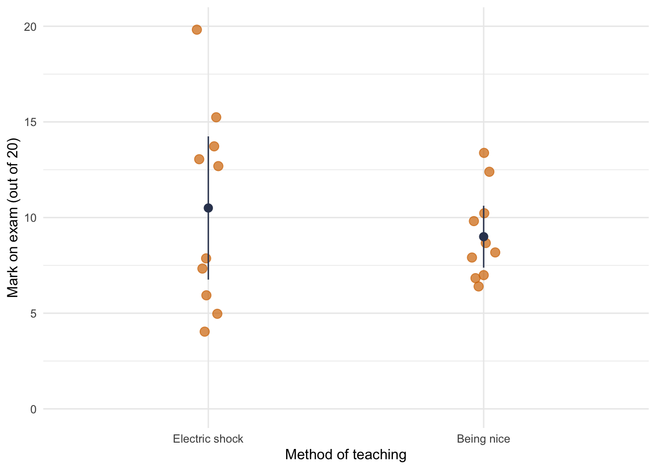
We can see that there was no significant main effect of method of teaching, F(1, 16) = 2.25, p = 0.153, indicating that when we ignore the sex of the participant both methods of teaching had similar effects on the results of the exam. This result is not surprising when we look at the graphed means because being nice (M = 9.0) and electric shock (M = 10.5) had similar means.
ggplot(teach_tib, aes(method, mark)) +
  geom_point(size = 3, position = position_jitter(width = 0.05), colour = ong, alpha = 0.7) +
  stat_summary(fun.data = "mean_cl_normal", geom = "pointrange", colour = blu_dk) +
  coord_cartesian(ylim = c(0, 20)) +
  labs(x = "Method of teaching", y = "Mark on exam (out of 20)") +
  theme_minimal()
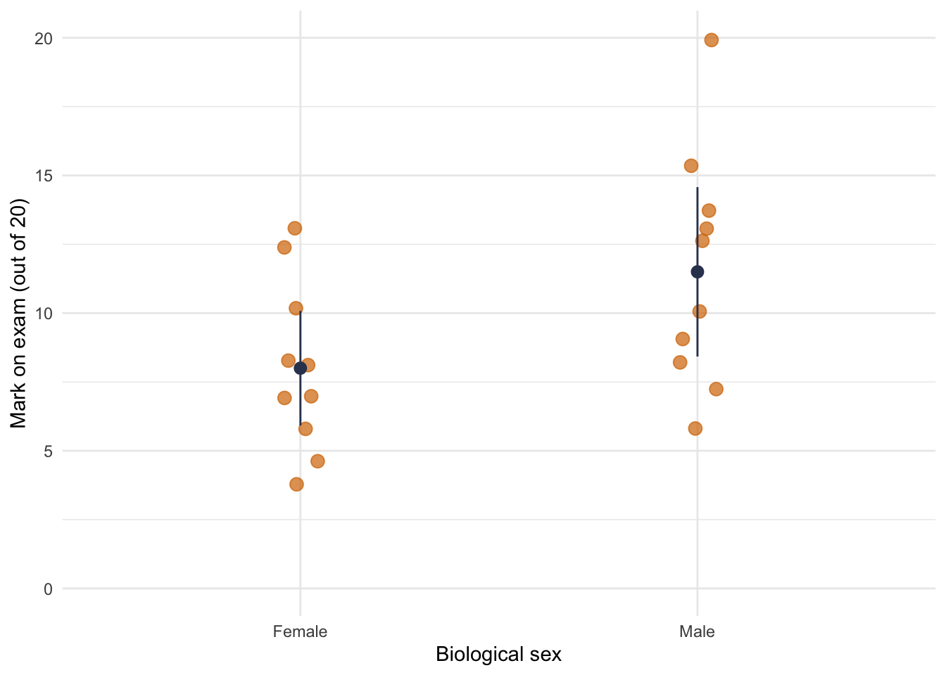
There was a significant main effect of the sex of the participant, F(1, 16) = 12.25, p < .01, indicating that if we ignore the method of teaching, men and women scored differently on the exam. If we look at the graphed means, we can see that on average men (M = 11.5) scored higher than women (M = 8.0).
ggplot(teach_tib, aes(sex, mark)) +
  geom_point(size = 3, position = position_jitter(width = 0.05),  colour = ong, alpha = 0.7) +
  stat_summary(fun.data = "mean_cl_normal", geom = "pointrange", colour = blu_dk) +
  coord_cartesian(ylim = c(0, 20)) +
  labs(x = "Biological sex", y = "Mark on exam (out of 20)") +
  theme_minimal()
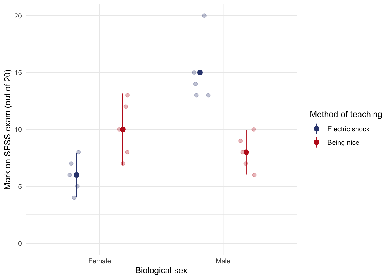
However, the main effect of sex is qualified by a significant interaction between sex and the method of teaching, F(1, 16) = 30.25, p < .001. The graphed means suggest that for men, using an electric shock resulted in higher exam scores than being nice, whereas for women, the being nice teaching method resulted in significantly higher exam scores than when an electric shock was used.
ggplot(teach_tib, aes(sex, mark, colour = method)) +
  geom_point(position = position_jitterdodge(dodge.width = 0.75, jitter.width = 0.3), size = 2, alpha = 0.3) +
  stat_summary(fun.data = "mean_cl_normal", geom = "pointrange", position = position_dodge(width = 0.75)) +
  coord_cartesian(ylim = c(0, 20)) +
  labs(x = "Biological sex", y = "Mark on SPSS exam (out of 20)", colour = "Method of teaching") +
  discovr::scale_color_prayer() +
  theme_minimal()
Task 13.6
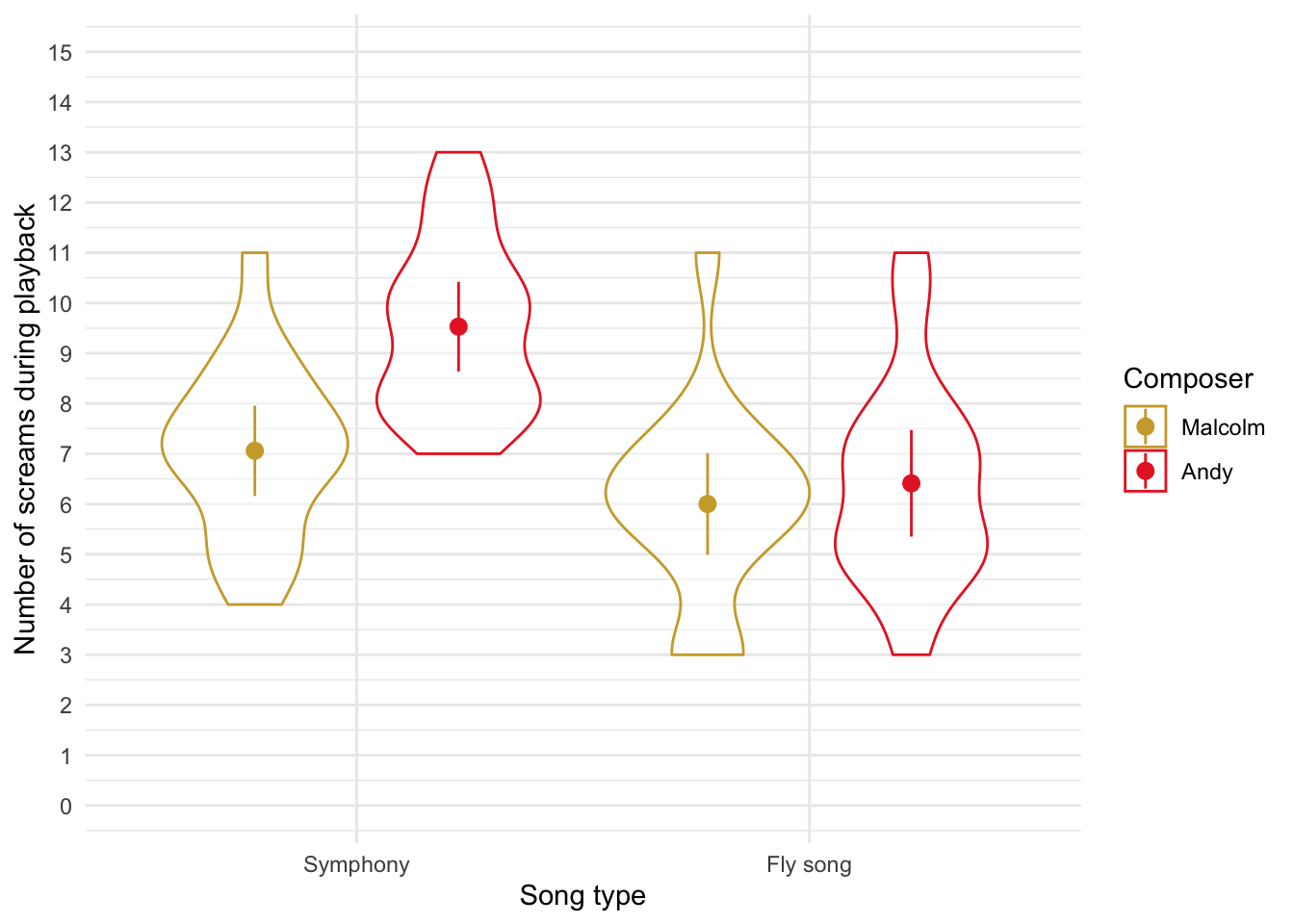
At the start of this Chapter I described a way of empirically researching whether I wrote better songs than my old bandmate Malcolm, and whether this depended on the type of song (a symphony or song about flies). The outcome variable was the number of screams elicited by audience members during the songs. Plot the data and fit a model to test my hypothesis that the type of song moderates which songwriter is preferred (escape.csv).
Load the data
To load the data from the CSV file (assuming you have set up a project folder as suggested in the book) and set the factor and its levels:
escape_tib <- readr::read_csv("../data/escape.csv") %>%
  dplyr::mutate(
    song_type = forcats::as_factor(song_type) %>% forcats::fct_relevel(., "Symphony"),
    songwriter = forcats::as_factor(songwriter) %>% forcats::fct_relevel(., "Malcolm")
  )
Alternative, load the data directly from the discovr package:
escape_tib <- discovr::escape
Plot the data
ggplot2::ggplot(escape_tib, aes(x = song_type, y = screams, colour = songwriter)) +
  geom_violin(alpha = 0.5) +
  stat_summary(fun.data = "mean_cl_normal", position = position_dodge(width = 0.9)) +
  coord_cartesian(ylim = c(0, 15)) +
  scale_y_continuous(breaks = seq(0, 15, 1)) +
  labs(y = "Number of screams during playback", x = "Song type", colour = "Composer") +
  discovr::scale_colour_pom() +
  theme_minimal()
The plot shows that after listening to an angle grinder both groups are angry. After listening to metal, the metal heads score low on anger but the pop fans score high. the reverse is true after listening to pop music.
Fitting the model using afex::aov_4()
escape_afx <- afex::aov_4(screams ~ song_type*songwriter + (1|id), data = escape_tib)
escape_afx
## Anova Table (Type 3 tests)
##
## Response: screams
##                 Effect    df  MSE         F  ges p.value
## 1            song_type 1, 64 3.55 20.87 *** .246   <.001
## 2           songwriter 1, 64 3.55   9.94 ** .134    .002
## 3 song_type:songwriter 1, 64 3.55    5.07 * .073    .028
## ---
## Signif. codes:  0 '***' 0.001 '**' 0.01 '*' 0.05 '+' 0.1 ' ' 1
Fitting the model using lm()
Both song_type and songwriter have only two levels, so we don’t need contrasts to test hypothesises, but we need orthogonal ones for our Type III sums of squares. Let’s use the built in contr.sum to set these.
Set contrasts:
contrasts(escape_tib$song_type) <- contr.sum(2)
contrasts(escape_tib$songwriter) <- contr.sum(2)
Fit the model and print Type III sums of squares:
escape_lm <- lm(screams ~ song_type*songwriter, data = escape_tib)
car::Anova(escape_lm, type = 3)
## Anova Table (Type III tests)
##
## Response: screams
##                      Sum Sq Df   F value    Pr(>F)
## (Intercept)          3574.3  1 1006.4141 < 2.2e-16 ***
## song_type              74.1  1   20.8737 2.293e-05 ***
## songwriter             35.3  1    9.9420   0.00246 **
## song_type:songwriter   18.0  1    5.0725   0.02775 *
## Residuals             227.3 64
## ---
## Signif. codes:  0 '***' 0.001 '**' 0.01 '*' 0.05 '.' 0.1 ' ' 1
Interpret the model
There was a significant main effect of songwriter, F(1, 64) = 9.94, p < .01. Using the estimated marginal means this effect indicates that when we ignore the type of song Andy’s songs elicited significantly more screams than those written by Malcolm.
emmeans::emmeans(escape_afx, "songwriter")
##  songwriter emmean    SE df lower.CL upper.CL
##  Malcolm      6.53 0.323 64     5.88     7.18
##  Andy         7.97 0.323 64     7.32     8.62
##
## Results are averaged over the levels of: song_type
## Confidence level used: 0.95
There was a significant main effect of the type of song, F(1, 64) = 20.87, p < .001. Using the estimated marginal means this effect indicates that symphonies elicited significantly more screams of agony than songs about flies.
emmeans::emmeans(escape_afx, "song_type")
##  song_type emmean    SE df lower.CL upper.CL
##  Symphony    8.29 0.323 64     7.65     8.94
##  Fly song    6.21 0.323 64     5.56     6.85
##
## Results are averaged over the levels of: songwriter
## Confidence level used: 0.95
The interaction was also significant, F(1, 64) = 5.07, p = 0.028. The graphed means (see earlier) suggest that although reactions to Malcolm’s and Andy’s songs were similar for the fly songs, they differed quite a bit for the symphonies (Andy’s symphony elicited more screams of torment than Malcolm’s). Therefore, although the main effect of songwriter suggests that Malcolm was a better songwriter than Andy, the interaction tells us that this effect is driven by Andy being poor at writing symphonies.
Let’s have a look at the simple effects. they confirm that the number of screams significantly differed between Malcolm and Andy’s symphonies, but not for their songs about flies.
emmeans::joint_tests(escape_afx, "song_type")
## song_type = Symphony:
##  model term df1 df2 F.ratio p.value
##  songwriter   1  64  14.609 0.0003
##
## song_type = Fly song:
##  model term df1 df2 F.ratio p.value
##  songwriter   1  64   0.406 0.5264
Task 13.7
Compute omega squared for the effects in Task 6 and report the results of the analysis.
Omega squared for models using aov_4() (for the model using lm() replace escape_afx with escape_lm)
effectsize::omega_squared(escape_afx, ci = 0.95, partial = FALSE)
## # Effect Size for ANOVA (Type III)
##
## Parameter            | Omega2 |       95% CI
## --------------------------------------------
## song_type            |   0.20 | [0.05, 0.36]
## songwriter           |   0.09 | [0.00, 0.24]
## song_type:songwriter |   0.04 | [0.00, 0.17]
We could report (remember if you’re using APA format to drop the leading zeros before p-values and ω2, for example report p = .035 instead of p = 0.035):
- The main effect of the type of song significantly affected screams elicited during that song, F(1, 64) = 20.87, p < .001, ω2 = 0.2, 95% CI [0.05, 0.36]; the two symphonies elicited significantly more screams of agony than the two songs about flies.
- The main effect of the songwriter significantly affected screams elicited during that song, F(1, 64) = 9.94, p < .01, ω2 = 0.09, 95% CI [0, 0.24]; Andy’s songs elicited significantly more screams of torment from the audience than Malcolm’s songs.
- The song type$\times$songwriter interaction was significant, F(1, 64) = 5.07, p = 0.028, ω2 = 0.04, 95% CI [0, 0.17]. Although reactions to Malcolm’s and Andy’s songs were similar for songs about a fly, Andy’s symphony elicited more screams of torment than Malcolm’s. This effect was trivially small.
Task 13.8
There are reports of increases in injuries related to playing games consoles. These injuries were attributed mainly to muscle and tendon strains. A researcher hypothesized that a stretching warm-up before playing would help lower injuries, and that athletes would be less susceptible to injuries because their regular activity makes them more flexible. She took 60 athletes and 60 non-athletes (athlete); half of them played on a Nintendo Switch and half watched others playing as a control (switch), and within these groups half did a 5-minute stretch routine before playing/watching whereas the other half did not (stretch). The outcome was a pain score out of 10 (where 0 is no pain, and 10 is severe pain) after playing for 4 hours (injury). Fit a model to test whether athletes are less prone to injury, and whether the prevention programme worked (switch.csv).
Load the data
To load the data from the CSV file (assuming you have set up a project folder as suggested in the book) and set the factor and its levels:
switch_tib <- readr::read_csv("../data/switch.csv") %>%
   dplyr::mutate(
    athlete = forcats::as_factor(athlete),
    stretch = forcats::as_factor(stretch),
    switch = forcats::as_factor(switch)
  )
Alternative, load the data directly from the discovr package:
switch_tib <- discovr::switch
Fitting the model using afex::aov_4()
switch_afx <- afex::aov_4(injury ~ athlete*stretch*switch + (1|id), data = switch_tib)
switch_afx
## Anova Table (Type 3 tests)
##
## Response: injury
##                   Effect     df  MSE         F  ges p.value
## 1                athlete 1, 112 1.53 64.82 *** .367   <.001
## 2                stretch 1, 112 1.53  11.05 ** .090    .001
## 3                 switch 1, 112 1.53 55.66 *** .332   <.001
## 4        athlete:stretch 1, 112 1.53      1.23 .011    .270
## 5         athlete:switch 1, 112 1.53 45.18 *** .287   <.001
## 6         stretch:switch 1, 112 1.53 14.19 *** .112   <.001
## 7 athlete:stretch:switch 1, 112 1.53    5.94 * .050    .016
## ---
## Signif. codes:  0 '***' 0.001 '**' 0.01 '*' 0.05 '+' 0.1 ' ' 1
Fitting the model using lm()
The variables athlete, switch and stretch have only two levels, so we don’t need contrasts to test hypothesises, but we need orthogonal ones for our Type III sums of squares. Let’s use the built in contr.sum to set these.
Set contrasts:
contrasts(switch_tib$athlete) <- contr.sum(2)
contrasts(switch_tib$stretch) <- contr.sum(2)
contrasts(switch_tib$switch) <- contr.sum(2)
Fit the model and print Type III sums of squares:
switch_lm <- lm(injury ~ athlete*stretch*switch, data = switch_tib)
car::Anova(switch_lm, type = 3)
## Anova Table (Type III tests)
##
## Response: injury
##                         Sum Sq  Df  F value    Pr(>F)
## (Intercept)            1003.41   1 656.9470 < 2.2e-16 ***
## athlete                  99.01   1  64.8223 9.595e-13 ***
## stretch                  16.87   1  11.0483 0.0012001 **
## switch                   85.01   1  55.6563 1.982e-11 ***
## athlete:stretch           1.88   1   1.2276 0.2702496
## athlete:switch           69.01   1  45.1808 7.869e-10 ***
## stretch:switch           21.68   1  14.1910 0.0002651 ***
## athlete:stretch:switch    9.08   1   5.9415 0.0163612 *
## Residuals               171.07 112
## ---
## Signif. codes:  0 '***' 0.001 '**' 0.01 '*' 0.05 '.' 0.1 ' ' 1
Interpret the model
There was a significant main effect of athlete, F(1, 112) = 64.82, p < .001. The EMMs show that, on average, athletes had significantly lower injury scores than non-athletes.
emmeans::emmeans(switch_afx, "athlete")
##  athlete     emmean   SE  df lower.CL upper.CL
##  Athlete       1.98 0.16 112     1.67     2.30
##  Non-athlete   3.80 0.16 112     3.48     4.12
##
## Results are averaged over the levels of: stretch, switch
## Confidence level used: 0.95
There was a significant main effect of stretching, F(1, 112) = 11.05, p < .01. The EMMs shows that stretching significantly decreased injury score compared to not stretching. However, the two-way interaction with athletes will show us that this is true only for athletes and non-athletes who played on the switch, not for those in the control group (you can also see this pattern in the three-way interaction graph). This is an example of how main effects can sometimes be misleading.
emmeans::emmeans(switch_afx, "stretch")
##  stretch       emmean   SE  df lower.CL upper.CL
##  Stretching      2.52 0.16 112     2.20     2.83
##  No stretching   3.27 0.16 112     2.95     3.58
##
## Results are averaged over the levels of: athlete, switch
## Confidence level used: 0.95
There was also a significant main effect of switch, F(1, 112) = 55.66, p < .001. The EMMs shows (not surprisingly) that playing on the switch resulted in a significantly higher injury score compared to watching other people playing on the switch (control).
emmeans::emmeans(switch_afx, "switch")
##  switch          emmean   SE  df lower.CL upper.CL
##  Playing switch    3.73 0.16 112     3.42     4.05
##  Watching switch   2.05 0.16 112     1.73     2.37
##
## Results are averaged over the levels of: athlete, stretch
## Confidence level used: 0.95
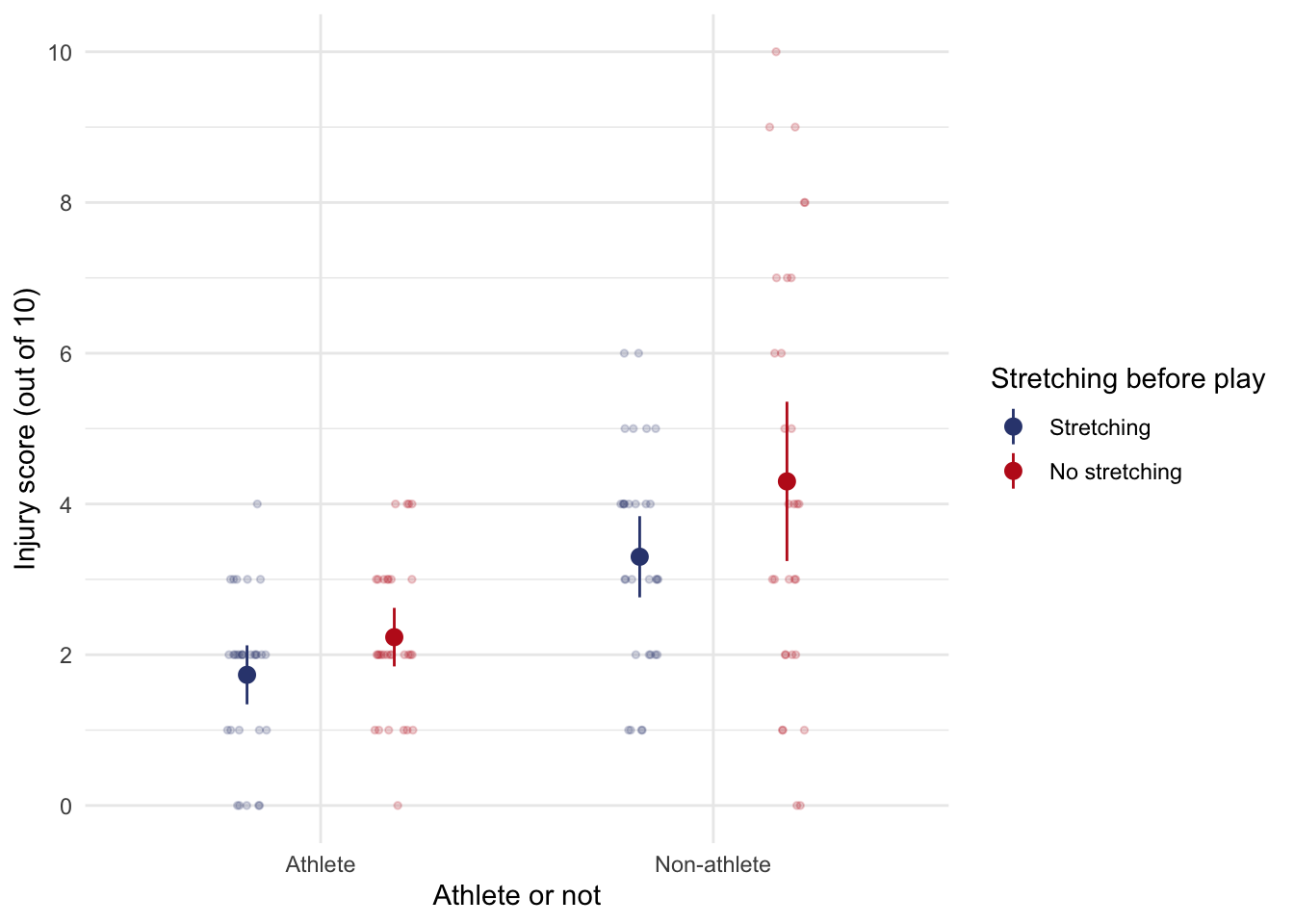
There was not a significant athlete by stretch interaction, F(1, 112) = 1.23, p = 0.27. The graph of the interaction effect shows that (not taking into account playing vs. watching the switch) while non-athletes had higher injury scores than athletes overall, stretching decreased the number of injuries in both athletes and non-athletes by roughly the same amount. Parallel lines usually indicate a non-significant interaction effect, and so it is not surprising that the interaction between stretch and athlete was non-significant.
ggplot(switch_tib, aes(athlete, injury, colour = stretch)) +
  geom_point(position = position_jitterdodge(dodge.width = 0.75, jitter.width = 0.2), size = 1, alpha = 0.2) +
  stat_summary(fun.data = "mean_cl_normal", position = position_dodge(width = 0.75)) +
  labs(x = "Athlete or not", y = "Injury score (out of 10)", colour = "Stretching before play") +
  discovr::scale_color_prayer() +
  coord_cartesian(ylim = c(0, 10)) +
  scale_y_continuous(breaks = seq(0, 10, 2)) +
  theme_minimal()
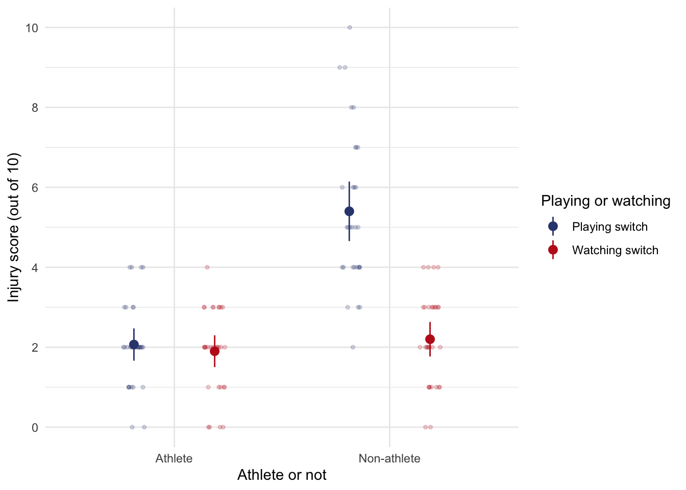
There was a significant athlete by switch interaction, F(1, 112) = 45.18, p < .001. The interaction graph shows that (not taking stretching into account) non-athletes had low injury scores when watching but high injury scores when playing whereas athletes had low injury scores when both playing and watching.
ggplot(switch_tib, aes(athlete, injury, colour = switch)) +
  geom_point(position = position_jitterdodge(dodge.width = 0.75, jitter.width = 0.2), size = 1, alpha = 0.2) +
  stat_summary(fun.data = "mean_cl_normal", position = position_dodge(width = 0.75)) +
  labs(x = "Athlete or not", y = "Injury score (out of 10)", colour = "Playing or watching") +
  discovr::scale_color_prayer() +
  coord_cartesian(ylim = c(0, 10)) +
  scale_y_continuous(breaks = seq(0, 10, 2)) +
  theme_minimal()
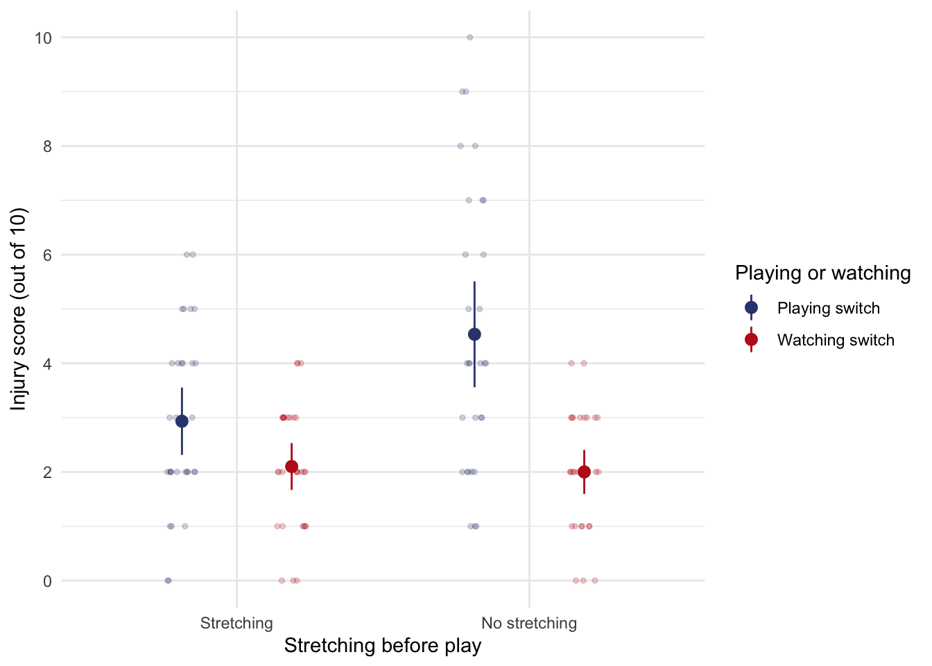
There was a significant stretch by switch interaction, F(1, 112) = 14.19, p < .001. The interaction graph shows that (not taking athlete into account) stretching before playing on the switch significantly decreased injury scores, but stretching before watching other people playing on the switch did not significantly reduce injury scores. This is not surprising as watching other people playing on the switch is unlikely to result in sports injury!
ggplot(switch_tib, aes(stretch, injury, colour = switch)) +
  geom_point(position = position_jitterdodge(dodge.width = 0.75, jitter.width = 0.2), size = 1, alpha = 0.2) +
  stat_summary(fun.data = "mean_cl_normal", position = position_dodge(width = 0.75)) +
  labs(x = "Stretching before play", y = "Injury score (out of 10)", colour = "Playing or watching") +
  discovr::scale_color_prayer() +
  coord_cartesian(ylim = c(0, 10)) +
  scale_y_continuous(breaks = seq(0, 10, 2)) +
  theme_minimal()
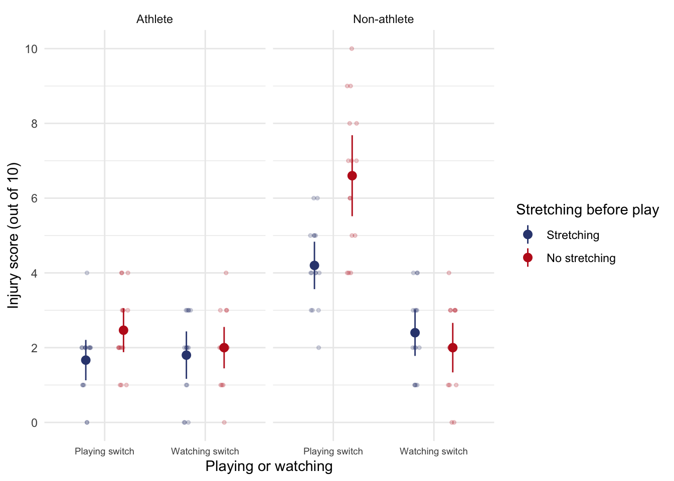
There was a significant athlete by stretch by switch interaction, F(1, 112) = 5.94, p = 0.016. What this actually means is that the effect of stretching and playing on the switch on injury score was different for athletes than it was for non-athletes. In the presence of this significant interaction it makes no sense to interpret the main effects. The interaction graph for this three-way effect shows that for athletes, stretching and playing on the switch has very little effect: their mean injury score is quite stable across the two conditions (whether they played on the switch or watched other people playing on the switch, stretched or did no stretching). However, for the non-athletes, watching other people play on the switch compared to not stretching and playing on the switch rapidly declines their mean injury score. The interaction tells us that stretching and watching rather than playing on the switch both result in a lower injury score and that this is true only for non-athletes. In short, the results show that athletes are able to minimize their injury level regardless of whether they stretch before exercise or not, whereas non-athletes only have to bend slightly and they get injured!
ggplot(switch_tib, aes(switch, injury, colour = stretch)) +
  geom_point(position = position_jitterdodge(dodge.width = 0.75, jitter.width = 0.2), size = 1, alpha = 0.2) +
  stat_summary(fun.data = "mean_cl_normal", position = position_dodge(width = 0.75)) +
  facet_wrap(~athlete) +
  labs(x = "Playing or watching", y = "Injury score (out of 10)", colour = "Stretching before play") +
  discovr::scale_color_prayer() +
  coord_cartesian(ylim = c(0, 10)) +
  scale_y_continuous(breaks = seq(0, 10, 2)) +
  theme_minimal() +
  theme(axis.text.x = element_text(size = rel(0.8)))
Task 13.9
A researcher was interested in what factors contributed to injuries resulting from game console use. She tested 40 participants who were randomly assigned to either an active or static game played on either a Nintendo Switch or Xbox One Kinect. At the end of the session their physical condition was evaluated on an injury severity scale. The data are in the file xbox.csv which contains the variables game (0 = static, 1 = active), console (0 = Switch, 1 = Xbox), and injury (a score ranging from 0 (no injury) to 20 (severe injury)). Fit a model to see whether injury severity is significantly predicted from the type of game, the type of console and their interaction
Load the data
To load the data from the CSV file (assuming you have set up a project folder as suggested in the book) and set the factor and its levels:
switch_tib <- readr::read_csv("../data/xbox.csv") %>%
   dplyr::mutate(
    game = forcats::as_factor(game),
    console = forcats::as_factor(console)
  )
Alternative, load the data directly from the discovr package:
xbox_tib <- discovr::xbox
Fitting the model using afex::aov_4()
xbox_afx <- afex::aov_4(injury ~ game*console + (1|id), data = xbox_tib)
xbox_afx
## Anova Table (Type 3 tests)
##
## Response: injury
##         Effect    df  MSE         F  ges p.value
## 1         game 1, 36 7.15 25.86 *** .418   <.001
## 2      console 1, 36 7.15    3.58 + .090    .067
## 3 game:console 1, 36 7.15    5.05 * .123    .031
## ---
## Signif. codes:  0 '***' 0.001 '**' 0.01 '*' 0.05 '+' 0.1 ' ' 1
Fitting the model using lm()
The variables game and console have only two levels, so we don’t need contrasts to test hypothesises, but we need orthogonal ones for our Type III sums of squares. Let’s use the built in contr.sum to set these.
Set contrasts:
contrasts(xbox_tib$game) <- contr.sum(2)
contrasts(xbox_tib$console) <- contr.sum(2)
Fit the model and print Type III sums of squares:
xbox_lm <- lm(injury ~ game*console, data = xbox_tib)
car::Anova(xbox_lm, type = 3)
## Anova Table (Type III tests)
##
## Response: injury
##              Sum Sq Df  F value    Pr(>F)
## (Intercept)  3240.0  1 453.1469 < 2.2e-16 ***
## game          184.9  1  25.8601 1.157e-05 ***
## console        25.6  1   3.5804   0.06653 .
## game:console   36.1  1   5.0490   0.03087 *
## Residuals     257.4 36
## ---
## Signif. codes:  0 '***' 0.001 '**' 0.01 '*' 0.05 '.' 0.1 ' ' 1
Interpret the model
There was a significant main effect of game, F(1, 36) = 25.86, p < .001. The EMMs show that, on average, injuries were significantly higher for active games than static ones.
emmeans::emmeans(xbox_afx, "game")
##  game   emmean    SE df lower.CL upper.CL
##  Active  11.15 0.598 36     9.94    12.36
##  Static   6.85 0.598 36     5.64     8.06
##
## Results are averaged over the levels of: console
## Confidence level used: 0.95
There was not a significant main effect of console, F(1, 36) = 3.58, p = 0.067. The mean number of injuries was not significantly different between xboix and switch games (but remember this effect collapses across active and static games).
emmeans::emmeans(xbox_afx, "console")
##  console  emmean    SE df lower.CL upper.CL
##  Xbox One    8.2 0.598 36     6.99     9.41
##  Switch      9.8 0.598 36     8.59    11.01
##
## Results are averaged over the levels of: game
## Confidence level used: 0.95
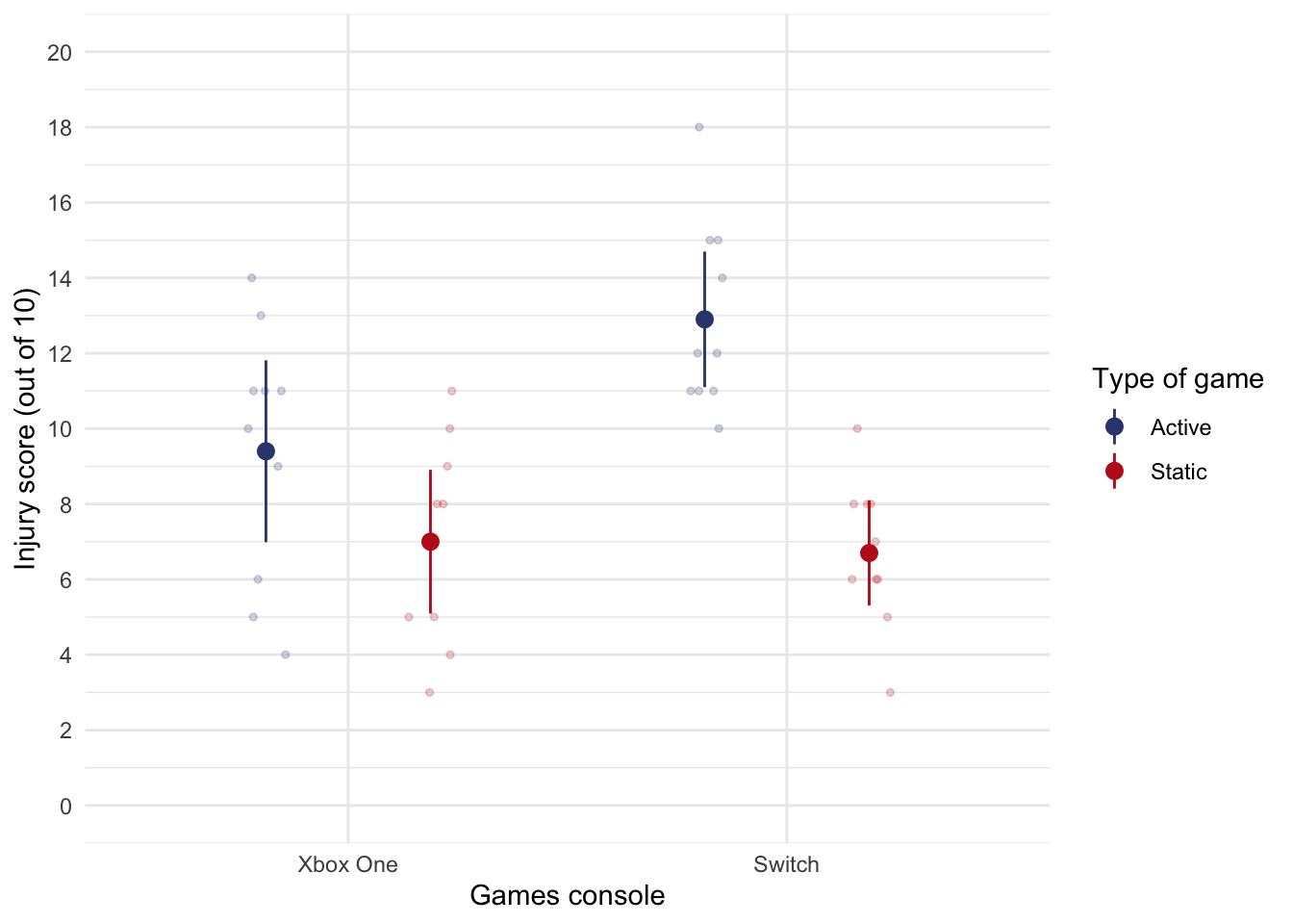
There was a significant game by console interaction, F(1, 36) = 5.05, p = 0.031. The interaction graph shows that for both consoles injuries were higher for active games compared to static ones, but this difference (the gap between the red and blue dots) is bigger for the switch than the xbox.
ggplot(xbox_tib, aes(console, injury, colour = game)) +
  geom_point(position = position_jitterdodge(dodge.width = 0.75, jitter.width = 0.2), size = 1, alpha = 0.2) +
  stat_summary(fun.data = "mean_cl_normal", position = position_dodge(width = 0.75)) +
  labs(x = "Games console", y = "Injury score (out of 10)", colour = "Type of game") +
  discovr::scale_color_prayer() +
  coord_cartesian(ylim = c(0, 20)) +
  scale_y_continuous(breaks = seq(0, 20, 2)) +
  theme_minimal()
Simple effects show that the difference between static and active games is just not significant for the xbox, but is very significantly different for the switch.
emmeans::joint_tests(xbox_afx, "console")
## console = Xbox One:
##  model term df1 df2 F.ratio p.value
##  game         1  36   4.028 0.0523
##
## console = Switch:
##  model term df1 df2 F.ratio p.value
##  game         1  36  26.881 <.0001