Smart Alex solutions Chapter 12

This document contains abridged sections from Discovering Statistics Using R and RStudio by Andy Field so there are some copyright considerations. You can use this material for teaching and non-profit activities but please do not meddle with it or claim it as your own work. See the full license terms at the bottom of the page.
Task 12.1
A few years back I was stalked. You’d think they could have found someone a bit more interesting to stalk, but apparently times were hard. It could have been a lot worse, but it wasn’t particularly pleasant. I imagined a world in which a psychologist tried two different therapies on different groups of stalkers (25 stalkers in each group – this variable is called therapy). To the first group he gave cruel-to-be-kind therapy (every time the stalkers followed him around, or sent him a letter, the psychologist attacked them with a cattle prod). The second therapy was Psychodyshamic therapy, in which stalkers were hypnotized and regressed into their childhood to discuss their penis (or lack of penis), their father’s penis, their dog’s penis, the seventh penis of a seventh penis, and any other penis that sprang to mind. The psychologist measured the number of hours stalking in one week both before (stalk_pre) and after (stalk_post) treatment. Analyse the effect of therapy on stalking behaviour after therapy, adjusting for the amount of stalking behaviour before therapy.
Load the data
To load the data from the CSV file (assuming you have set up a project folder as suggested in the book) and set the factor and its levels:
stalk_tib <- readr::read_csv("../data/stalker.csv") %>%
   dplyr::mutate(
    therapy = forcats::as_factor(therapy) %>% forcats::fct_relevel(., "Cruel to be kind")
  )
Alternative, load the data directly from the discovr package:
stalk_tib <- discovr::stalker
Fit the model
First, test whether the number of hours spent stalking before therapy (our covariate) is independent of the type of therapy (our predictor variable):
pre_lm <- lm(stalk_pre ~ therapy, data = stalk_tib)

anova(pre_lm) %>%
  parameters::model_parameters()
## Parameter | Sum_Squares | df | Mean_Square |    F |     p
## ---------------------------------------------------------
## therapy   |        7.22 |  1 |        7.22 | 0.06 | 0.804
## Residuals |     5555.36 | 48 |      115.74 |      |
The output shows that the main effect of therapy is not significant, F(1, 48) = 0.06, p = 0.804, which shows that the average level of stalking behaviour before therapy was roughly the same in the two therapy groups. In other words, the mean number of hours spent stalking before therapy is not significantly different in the cruel-to-be-kind and Psychodyshamic therapy groups. This result is good news for using stalking behaviour before therapy as a covariate in the analysis.
The categorical predictor (therapy) only has two levels/categories so we don’t need to set contrasts. We can fit the main model as:
stalk_lm <- lm(stalk_post ~ stalk_pre + therapy, data = stalk_tib)
car::Anova(stalk_lm, type = 3)
## Anova Table (Type III tests)
##
## Response: stalk_post
##             Sum Sq Df F value    Pr(>F)
## (Intercept)   10.1  1  0.1158   0.73520
## stalk_pre   4414.6  1 50.4621 5.692e-09 ***
## therapy      480.3  1  5.4898   0.02341 *
## Residuals   4111.7 47
## ---
## Signif. codes:  0 '***' 0.001 '**' 0.01 '*' 0.05 '.' 0.1 ' ' 1
The output shows that the covariate significantly predicts the outcome variable, so the hours spent stalking after therapy depend on the extent of the initial problem (i.e. the hours spent stalking before therapy). More interesting is that after adjusting for the effect of initial stalking behaviour, the effect of therapy is significant. To interpret the results of the main effect of therapy we look at the adjusted means:
modelbased::estimate_means(stalk_lm, fixed = "stalk_pre")
## therapy          | stalk_pre |  Mean |   SE |         95% CI
## ------------------------------------------------------------
## Cruel to be kind |     65.22 | 55.30 | 1.87 | [51.53, 59.06]
## Psychodyshamic   |     65.22 | 61.50 | 1.87 | [57.74, 65.27]
The adjusted means tell us that stalking behaviour was lower after the therapy involving the cattle prod than after Psychodyshamic therapy (after adjusting for baseline stalking).
To interpret the covariate look at the parameter estimates:
broom::tidy(stalk_lm, conf.int = TRUE) %>%
  knitr::kable(digits = 2)
| term | estimate | std.error | statistic | p.value | conf.low | conf.high |
|---|---|---|---|---|---|---|
| (Intercept) | -2.84 | 8.35 | -0.34 | 0.74 | -19.64 | 13.96 |
| stalk_pre | 0.89 | 0.13 | 7.10 | 0.00 | 0.64 | 1.14 |
| therapyPsychodyshamic | 6.20 | 2.65 | 2.34 | 0.02 | 0.88 | 11.53 |
The parameter estimate shows that there is a positive relationship between stalking pre-therapy and post-therapy, b = 0.89. That is, higher stalking levels pre-therapy corresponded with higher levels post therapy.
Check model diagnostics
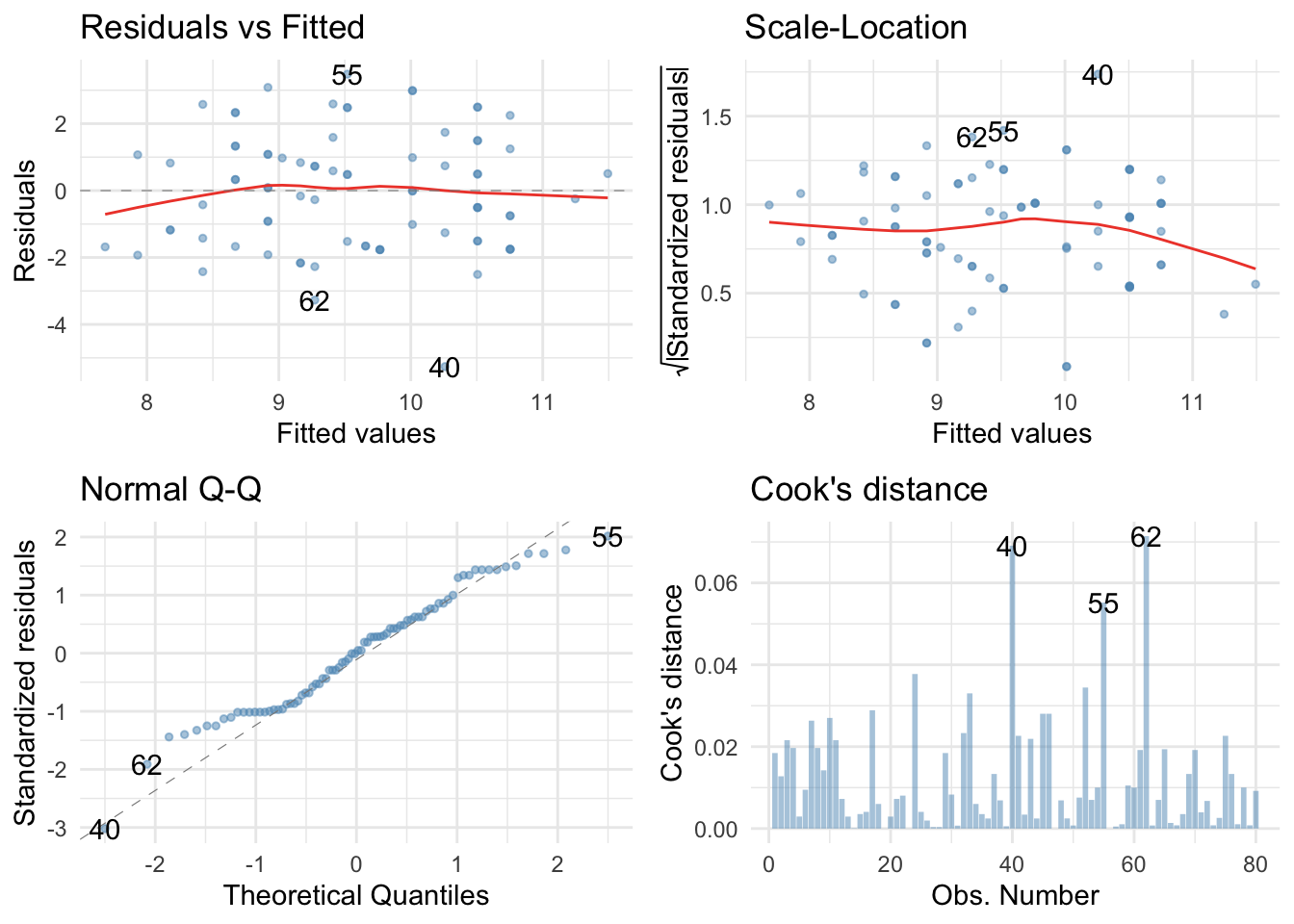
We can get some basic diagnostic plots as follows:
library(ggfortify) # remember to load this package
ggplot2::autoplot(stalk_lm,
                  which = c(1, 3, 2, 4),
                  colour = "#5c97bf",
                  smooth.colour = "#ef4836",
                  alpha = 0.5,
                  size = 1) +
  theme_minimal()
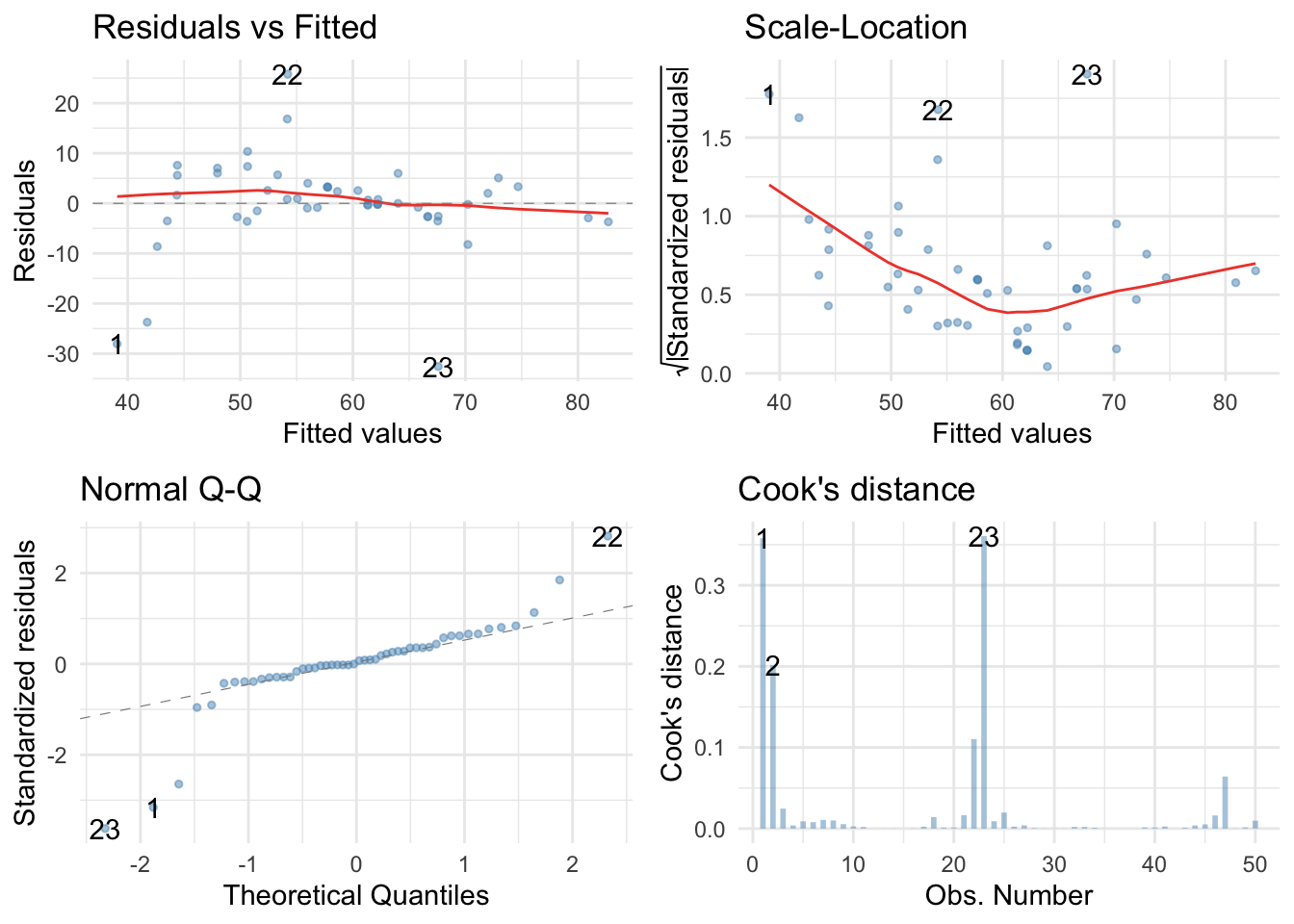 The Q-Q plot suggests non-normal residuals and the residual vs fitted plot and the scale-location plot suggest heterogeneity of variance. Which brings us to Task 2.
Task 12.2
Fit a robust model for Task 1
We should fit a robust model. Because there was a problem with normality of residuals (which affects parameter estimates) and heteroscedasticity (which affects significance tests and confidence intervals) we should use:
stalk_rob <- robust::lmRob(stalk_post ~ stalk_pre + therapy, data = stalk_tib)
summary(stalk_rob)
##
## Call:
## robust::lmRob(formula = stalk_post ~ stalk_pre + therapy, data = stalk_tib)
##
## Residuals:
##        Min         1Q     Median         3Q        Max
## -34.783005  -2.426286   0.003723   1.894398  21.643705
##
## Coefficients:
##                       Estimate Std. Error t value Pr(>|t|)
## (Intercept)            9.60233    3.20285   2.998  0.00433 **
## stalk_pre              0.76178    0.04596  16.575  < 2e-16 ***
## therapyPsychodyshamic  1.61503    0.92560   1.745  0.08755 .
## ---
## Signif. codes:  0 '***' 0.001 '**' 0.01 '*' 0.05 '.' 0.1 ' ' 1
##
## Residual standard error: 3.207 on 47 degrees of freedom
## Multiple R-Squared: 0.5159
##
## Test for Bias:
##             statistic p-value
## M-estimate      6.588 0.08627
## LS-estimate     9.291 0.02567
The robust model, contrary to the non-robust model, suggests that after adjusting for pre-therapy levels of stalking there is no significant difference between the types of treatments. Note also that the parameter estimate for the type of therapy has fallen from 6.2 (non-robust) to 1.6 (robust) suggesting a much smaller effect when robust estimation is used.
Task 12.3
A marketing manager tested the benefit of soft drinks for curing hangovers. He took 15 people and got them drunk. The next morning as they awoke, dehydrated and feeling as though they’d licked a camel’s sandy feet clean with their tongue, he gave five of them water to drink, five of them Lucozade (a very nice glucose-based UK drink) and the remaining five a leading brand of cola (this variable is called drink). He measured how well they felt (on a scale from 0 = I feel like death to 10 = I feel really full of beans and healthy) two hours later (this variable is called well). He measured how drunk the person got the night before on a scale of 0 = as sober as a nun to 10 = flapping about like a haddock out of water on the floor in a puddle of their own vomit (hangover.csv). Fit a model to see whether people felt better after different drinks when adjusting for how drunk they were the night before.
Load the data
To load the data from the CSV file (assuming you have set up a project folder as suggested in the book) and set the factor and its levels:
cure_tib <- readr::read_csv("../data/hangover.csv") %>%
   dplyr::mutate(
    drink = forcats::as_factor(drink) %>% forcats::fct_relevel(., "Water", "Lucozade", "Cola")
  )
Alternative, load the data directly from the discovr package:
cure_tib <- discovr::hangover
Set contrasts
We have three levels of drink (water, Lucozade, Cola). Two of these drinks contain sugar/glucose, so water is a control. Therefore, we could reasonable set a contrast that compares ‘sugary drinks’ to water, and then a second contrast that compares the two sugary drinks. The order of the levels are water, Lucozade, “Cola”, which we can confirm by executing:
levels(cure_tib$drink)
## [1] "Water" "Lucozade" "Cola"
Therefore, we’d set these contrasts as:
sugar_vs_none <- c(-2/3, 1/3, 1/3)
lucoz_vs_cola <- c(0, -1/2, 1/2)

contrasts(cure_tib$drink) <- cbind(sugar_vs_none, lucoz_vs_cola)
contrasts(cure_tib$drink) # execute to check/view the contrast
##          sugar_vs_none lucoz_vs_cola
## Water       -0.6666667           0.0
## Lucozade     0.3333333          -0.5
## Cola         0.3333333           0.5
Fit the model
First, let’s test that the predictor variable (drink) and the covariate (drunk) are independent:
drunk_lm <- lm(drunk ~ drink, data = cure_tib)

anova(drunk_lm) %>%
  parameters::model_parameters()
## Parameter | Sum_Squares | df | Mean_Square |    F |     p
## ---------------------------------------------------------
## drink     |        8.40 |  2 |        4.20 | 1.35 | 0.295
## Residuals |       37.20 | 12 |        3.10 |      |
The output shows that the main effect of drink is not significant, F(2, 12) = 1.35, p = 0.295, which shows that the average level of drunkenness the night before was roughly the same in the three drink groups. This result is good news for using the variable drunk as a covariate in the analysis.
We can fit the main model as:
cure_lm <- lm(well ~ drunk + drink, data = cure_tib)
car::Anova(cure_lm, type = 3)
## Anova Table (Type III tests)
##
## Response: well
##              Sum Sq Df  F value    Pr(>F)
## (Intercept) 145.006  1 361.4557 9.197e-10 ***
## drunk        11.187  1  27.8860   0.00026 ***
## drink         3.464  2   4.3177   0.04130 *
## Residuals     4.413 11
## ---
## Signif. codes:  0 '***' 0.001 '**' 0.01 '*' 0.05 '.' 0.1 ' ' 1
The output shows that the covariate significantly predicts the outcome variable, so the drunkenness of the person influenced how well they felt the next day. What’s more interesting is that after adjusting for the effect of drunkenness, the effect of drink is significant. Let’s look at the parameter estimates:
broom::tidy(cure_lm, conf.int = TRUE) %>%
  knitr::kable(digits = 3)
| term | estimate | std.error | statistic | p.value | conf.low | conf.high |
|---|---|---|---|---|---|---|
| (Intercept) | 7.398 | 0.389 | 19.012 | 0.000 | 6.541 | 8.254 |
| drunk | -0.548 | 0.104 | -5.281 | 0.000 | -0.777 | -0.320 |
| drinksugar_vs_none | 0.635 | 0.348 | 1.824 | 0.095 | -0.131 | 1.402 |
| drinklucoz_vs_cola | -0.987 | 0.442 | -2.233 | 0.047 | -1.960 | -0.014 |
From these estimates we could conclude that there is a negative relationship between how drunk you got and how well you felt after the ‘cure’: that is, the more drunk you got, the less well you felt the following day.
We can also see that the cola and water groups have statistically similar means whereas the cola and Lucozade groups have significantly different means. Let’s unpick this with the adjusted means:
modelbased::estimate_means(cure_lm, fixed = "drunk")
## drink    | drunk | Mean |   SE |       95% CI
## ---------------------------------------------
## Water    |  3.40 | 5.11 | 0.28 | [4.48, 5.73]
## Lucozade |  3.40 | 6.24 | 0.30 | [5.59, 6.89]
## Cola     |  3.40 | 5.25 | 0.30 | [4.59, 5.92]
The adjusted means show that people felt a lot more well in the Lucozade group (than both the water and cola groups). In fact, this finding explains the pattern of significance for the contrasts: because the Cola group has a very similar mean to the Water group, the combined mean of the Lucozade and Cola groups is also quite similar to the mean for water. The Cola mean ‘drags down’ the mean for ‘sugary drinks’. This is evident from the second contrast that shows that Lucozade drinkers had a significantly higher mean than Cola drinkers.
Check model diagnostics
We can get some basic diagnostic plots as follows:
library(ggfortify) # remember to load this package
ggplot2::autoplot(cure_lm,
                  which = c(1, 3, 2, 4),
                  colour = "#5c97bf",
                  smooth.colour = "#ef4836",
                  alpha = 0.5,
                  size = 1) +
  theme_minimal()
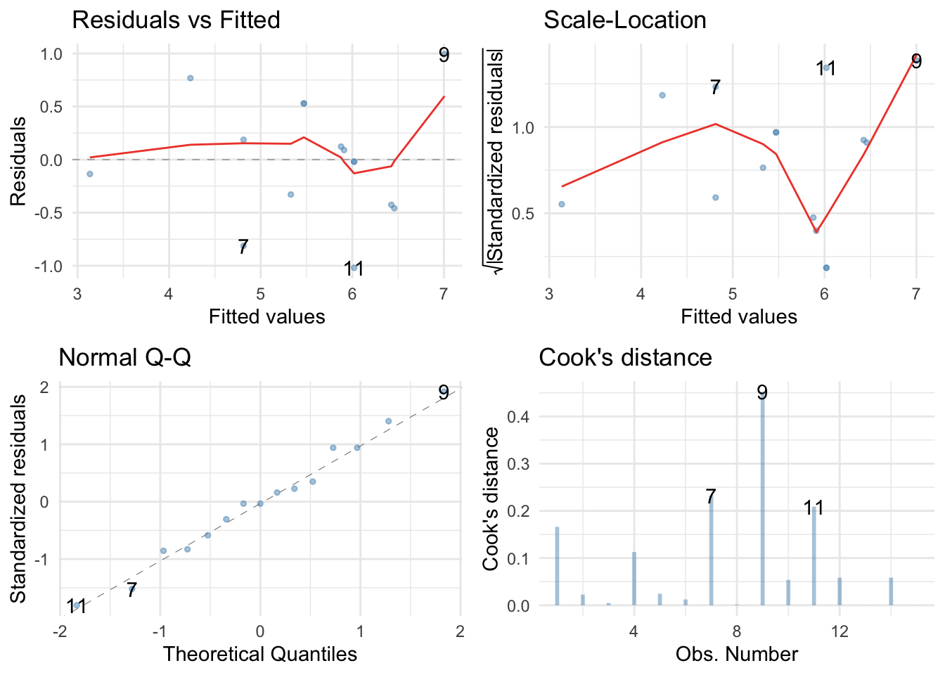 The Q-Q plot suggests normal residuals but the residual vs fitted plot and the scale-location plot suggest heterogeneity of variance.
We should fit a robust model. Because there was a problem with heteroscedasticity we can use a model that applies heteroscedasticity-consistent standard errors:
parameters::model_parameters(cure_lm, robust = TRUE, vcov.type = "HC4", digits = 3)
## Parameter          | Coefficient |    SE |         95% CI |      t | df |      p
## --------------------------------------------------------------------------------
## (Intercept)        |       7.398 | 0.506 | [ 6.28,  8.51] | 14.620 | 11 | < .001
## drunk              |      -0.548 | 0.127 | [-0.83, -0.27] | -4.302 | 11 | 0.001
## drinksugar_vs_none |       0.635 | 0.364 | [-0.17,  1.44] |  1.744 | 11 | 0.109
## drinklucoz_vs_cola |      -0.987 | 0.603 | [-2.32,  0.34] | -1.636 | 11 | 0.130
The robust model, contrary to the non-robust model, suggests that after adjusting for how much was drunk there are no significant differences in wellness between the groups who had different drinks as hangover cures.
Task 12.4
Compute effect sizes for Task 3 and report the results.
The effect sizes for the main effect of drink can be calculated as follows:
car::Anova(cure_lm, type = 3) %>%
  effectsize::omega_squared(ci = 0.95)
## Parameter | Omega2 (partial) |        95% CI
## --------------------------------------------
## drunk     |             0.64 | [ 0.25, 0.83]
## drink     |             0.31 | [-0.17, 0.63]
We could report the results as follows:
- The covariate, drunkenness, was significantly related to the how ill the person felt the next day, F(1, 11) = 27.89, p < 0.001, $ \omega_p^2 $ = 0.64. There was also a significant effect of the type of drink on how well the person felt after adjusting for how drunk they were the night before, F(2, 11) = 4.32, p = 0.041, $ \omega_p^2 $ = 0.44.
Robust planned contrasts using HC4 heteroscedasticity-consistent standard errors showed that having a sugary drink did not significantly affect wellness compared to water, $ b = 0.64 \ [-0.17, 1.44]\text{, } t(11) = 1.74\text{, } p = 0.109 $. Drinking Lucozade also did not significantly affect wellness compared to Cola, $ b = -0.99 \ [-2.32, 0.34]\text{, } t(11) = -1.64\text{, } p = 0.130 $.
Task 12.5
The highlight of the elephant calendar is the annual elephant soccer event in Nepal (google search it). A heated argument burns between the African and Asian elephants. In 2010, the president of the Asian Elephant Football Association, an elephant named Boji, claimed that Asian elephants were more talented than their African counterparts. The head of the African Elephant Soccer Association, an elephant called Tunc, issued a press statement that read ‘I make it a matter of personal pride never to take seriously any remark made by something that looks like an enormous scrotum’. I was called in to settle things. I collected data from the two types of elephants (elephant) over a season and recorded how many goals each elephant scored (goals) and how many years of experience the elephant had (experience). Analyse the effect of the type of elephant on goal scoring, covarying for the amount of football experience the elephant has (elephooty.csv).
Load the data
To load the data from the CSV file (assuming you have set up a project folder as suggested in the book) and set the factor and its levels:
ele_tib <- readr::read_csv("../data/elephooty.csv") %>%
  dplyr::mutate(
    elephant = forcats::as_factor(elephant) %>% forcats::fct_relevel(., "Asian", "African")
  )
Alternative, load the data directly from the discovr package:
ele_tib <- discovr::elephooty
Fit the model
First, let’s check that the predictor variable (elephant) and the covariate (experience) are independent:
exp_lm <- lm(experience ~ elephant, data = ele_tib)

anova(exp_lm) %>%
  parameters::model_parameters()
## Parameter | Sum_Squares |  df | Mean_Square |    F |     p
## ----------------------------------------------------------
## elephant  |        4.03 |   1 |        4.03 | 1.38 | 0.242
## Residuals |      343.93 | 118 |        2.91 |      |
The output shows that the main effect of elephant is not significant, F(1, 118) = 1.38, p = 0.24, which shows that the average level of prior football experience was roughly the same in the two elephant groups. This result is good news for using the variable experience as a covariate in the analysis.
The categorical predictor (elephant) only has two levels/categories so we don’t need to set contrasts. We can fit the main model as:
ele_lm <- lm(goals ~ experience + elephant, data = ele_tib)
car::Anova(ele_lm, type = 3)
## Anova Table (Type III tests)
##
## Response: goals
##             Sum Sq  Df F value    Pr(>F)
## (Intercept)  84.24   1 25.8825 1.397e-06 ***
## experience   32.32   1  9.9306  0.002065 **
## elephant     27.95   1  8.5887  0.004069 **
## Residuals   380.80 117
## ---
## Signif. codes:  0 '***' 0.001 '**' 0.01 '*' 0.05 '.' 0.1 ' ' 1
The output shows that the experience of the elephant significantly predicted how many goals they scored, F(1, 117) = 9.93, p = 0.002. After adjusting for the effect of experience, the effect of elephant is also significant. In other words, African and Asian elephants differed significantly in the number of goals they scored, F(1, 117) = 8.59, p = 0.004.
modelbased::estimate_means(ele_lm, fixed = "experience")
## elephant | experience | Mean |   SE |       95% CI
## --------------------------------------------------
## Asian    |       4.18 | 3.59 | 0.23 | [3.13, 4.05]
## African  |       4.18 | 4.56 | 0.23 | [4.10, 5.02]
The adjusted means tell us, specifically, that African elephants scored significantly more goals than Asian elephants after adjusting for prior experience
To interpret the covariate look at the parameter estimates:
broom::tidy(ele_lm, conf.int = TRUE) %>%
  knitr::kable(digits = 2)
| term | estimate | std.error | statistic | p.value | conf.low | conf.high |
|---|---|---|---|---|---|---|
| (Intercept) | 2.31 | 0.45 | 5.09 | 0 | 1.41 | 3.21 |
| experience | 0.31 | 0.10 | 3.15 | 0 | 0.11 | 0.50 |
| elephantAfrican | 0.97 | 0.33 | 2.93 | 0 | 0.31 | 1.63 |
The parameter estimate shows that there is a positive relationship between the two variables: the more prior football experience the elephant had, the more goals they scored in the season, b = 0.31.
Check model diagnostics
We can get some basic diagnostic plots as follows:
library(ggfortify) # remember to load this package
ggplot2::autoplot(ele_lm,
                  which = c(1, 3, 2, 4),
                  colour = "#5c97bf",
                  smooth.colour = "#ef4836",
                  alpha = 0.5,
                  size = 1) +
  theme_minimal()
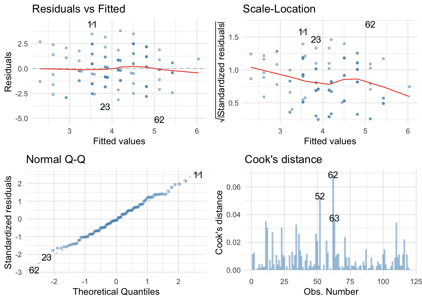 The Q-Q plot suggests normal residuals and the residual vs fitted plot suggest homogeneity of variance. However, the scale-location plot suggests heterogeneity (possibly). We could do a sensitivity analysis by applying heteroscedasticity-consistent standard errors to the tests of parameters:
parameters::model_parameters(ele_lm, robust = TRUE, vcov.type = "HC4", digits = 3)
## Parameter          | Coefficient |    SE |       95% CI |     t |  df |      p
## ------------------------------------------------------------------------------
## (Intercept)        |       2.307 | 0.456 | [1.40, 3.21] | 5.056 | 117 | < .001
## experience         |       0.307 | 0.089 | [0.13, 0.48] | 3.451 | 117 | < .001
## elephant [African] |       0.971 | 0.329 | [0.32, 1.62] | 2.948 | 117 | 0.004
Both effects are still highly significant using robust standard errors. Happy days.
Task 12.6
In Chapter 1 (Task 6) we looked at data from people who had been forced to marry goats and dogs and measured their life satisfaction and, also, how much they like animals (animal_bride.csv). Fit a model predicting life satisfaction from the type of animal to which a person was married and their animal liking score (covariate).
Load the data
To load the data from the CSV file (assuming you have set up a project folder as suggested in the book) and set the factor and its levels:
goat_tib <- readr::read_csv("../data/goat_or_dog.csv") %>%
  dplyr::mutate(
    wife = forcats::as_factor(wife)
  )
Alternative, load the data directly from the discovr package:
goat_tib <- discovr::animal_bride
Fit the model
First, check that the predictor variable (wife) and the covariate (animal) are independent:
animal_lm <- lm(animal ~ wife, data = goat_tib)

anova(animal_lm) %>%
  parameters::model_parameters()
## Parameter | Sum_Squares | df | Mean_Square |    F |     p
## ---------------------------------------------------------
## wife      |       14.70 |  1 |       14.70 | 0.06 | 0.812
## Residuals |     4520.50 | 18 |      251.14 |      |
The output shows that the main effect of wife is not significant, F(1, 18) = 0.06, p = 0.81, which shows that the average level of love of animals was roughly the same in the two type of animal wife groups. This result is good news for using the variable love of animals as a covariate in the analysis.
The categorical predictor (wife) only has two levels/categories so we don’t need to set contrasts. We can fit the main model as:
goat_lm <- lm(life_satisfaction ~ animal + wife, data = goat_tib)
car::Anova(goat_lm, type = 3)
## Anova Table (Type III tests)
##
## Response: life_satisfaction
##              Sum Sq Df F value    Pr(>F)
## (Intercept)  991.06  1  7.7174 0.0128876 *
## animal      1325.40  1 10.3208 0.0051071 **
## wife        2112.10  1 16.4468 0.0008223 ***
## Residuals   2183.14 17
## ---
## Signif. codes:  0 '***' 0.001 '**' 0.01 '*' 0.05 '.' 0.1 ' ' 1
The output shows that love of animals significantly predicted life satisfaction, F(1, 17) = 10.32, p = 0.005. After adjusting for the effect of love of animals, the effect of animal is also significant. In other words, life satisfaction differed significantly in those married to goats compared to those married to dogs, F(1, 17) = 16.45, p = 0.001.
To interpret the results of the main effect of therapy we look at the adjusted means:
modelbased::estimate_means(goat_lm, fixed = "animal")
## wife | animal |  Mean |   SE |         95% CI
## ---------------------------------------------
## Goat |  36.20 | 38.55 | 3.27 | [31.64, 45.45]
## Dog  |  36.20 | 59.56 | 4.01 | [51.10, 68.02]
The adjusted means tell us, specifically, that life satisfaction was significantly higher in those married to dogs. (My spaniel would like it on record that this result is obvious because, as he puts it, ‘dogs are fucking cool’.)
To interpret the covariate look at the parameter estimates:
broom::tidy(goat_lm, conf.int = TRUE) %>%
  knitr::kable(digits = 2)
| term | estimate | std.error | statistic | p.value | conf.low | conf.high |
|---|---|---|---|---|---|---|
| (Intercept) | 18.94 | 6.82 | 2.78 | 0.01 | 4.56 | 33.33 |
| animal | 0.54 | 0.17 | 3.21 | 0.01 | 0.19 | 0.90 |
| wifeDog | 21.01 | 5.18 | 4.06 | 0.00 | 10.08 | 31.94 |
The parameter estimate shows that there is a positive relationship, b = 0.54. The greater ones love of animals, the greater ones life satisfaction.
Check model diagnostics
We can get some basic diagnostic plots as follows:
library(ggfortify) # remember to load this package
ggplot2::autoplot(goat_lm,
                  which = c(1, 3, 2, 4),
                  colour = "#5c97bf",
                  smooth.colour = "#ef4836",
                  alpha = 0.5,
                  size = 1) +
  theme_minimal()
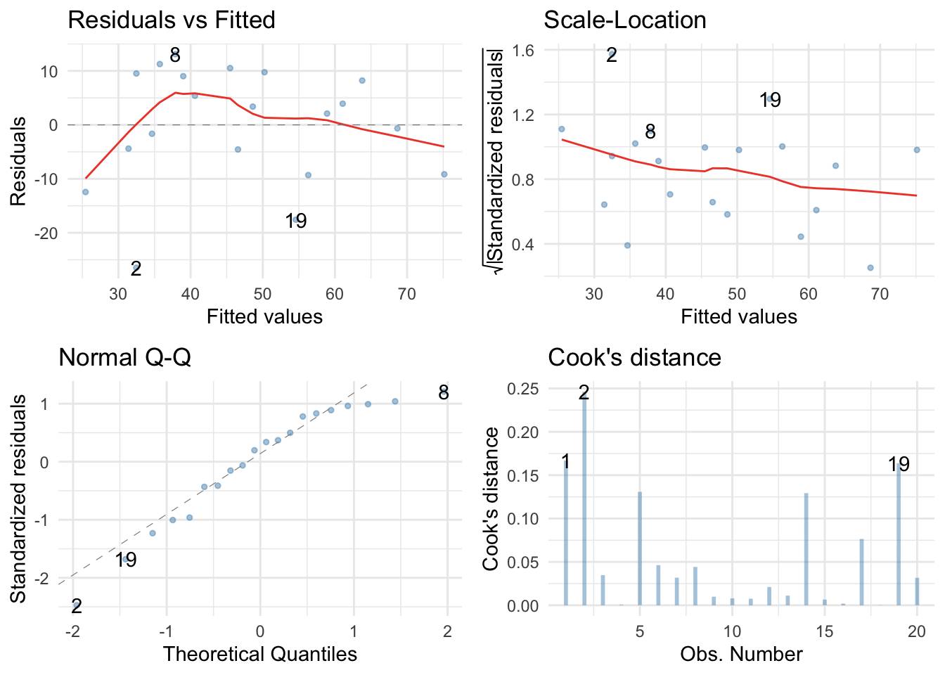 Holy shit, these are a mess. The Q-Q plot suggests non-normal residuals and the residual vs fitted plot and the scale-location plot suggest heterogeneity of variance.
Robust model
Let’s fit a robust model. Because there was a problem with normality of residuals (which affects parameter estimates) and heteroscedasticity (which affects significance tests and confidence intervals) we should use:
goat_rob <- robust::lmRob(life_satisfaction ~ animal + wife, data = goat_tib)
summary(goat_rob)
##
## Call:
## robust::lmRob(formula = life_satisfaction ~ animal + wife, data = goat_tib)
##
## Residuals:
##      Min       1Q   Median       3Q      Max
## -33.8602  -6.2417  -0.4648   2.8888   9.1646
##
## Coefficients:
##             Estimate Std. Error t value Pr(>|t|)
## (Intercept)  32.5945     5.5977   5.823 2.04e-05 ***
## animal        0.2906     0.1293   2.249   0.0381 *
## wifeDog      19.5825     3.8330   5.109 8.73e-05 ***
## ---
## Signif. codes:  0 '***' 0.001 '**' 0.01 '*' 0.05 '.' 0.1 ' ' 1
##
## Residual standard error: 8.129 on 17 degrees of freedom
## Multiple R-Squared: 0.4487
##
## Test for Bias:
##             statistic p-value
## M-estimate      3.209  0.3605
## LS-estimate     2.172  0.5376
Both effects are still significant and can be interpreted as for the non-robust model.
Task 12.7
Compute and interpret Bayes factors for the effects in Task 6.
goatcov_bf <-  BayesFactor::lmBF(formula = life_satisfaction ~ animal, data = goat_tib, rscaleFixed = "medium", rscaleCont = "medium")
goatcov_bf
## Bayes factor analysis
## --------------
## [1] animal : 3.064524 ±0%
##
## Against denominator:
##   Intercept only
## ---
## Bayes factor type: BFlinearModel, JZS
goat_bf <-  BayesFactor::lmBF(formula = life_satisfaction ~ animal + wife, data = goat_tib, rscaleCont = "medium", rscaleFixed = "medium")

goat_bf/goatcov_bf
## Bayes factor analysis
## --------------
## [1] animal + wife : 33.20849 ±0.81%
##
## Against denominator:
##   life_satisfaction ~ animal
## ---
## Bayes factor type: BFlinearModel, JZS
The output tells us that the data are 3.06 times more likely under the alternative hypothesis (life satisfaction is predicted from love of animals) than under the null (love of animals does not predict life satisfaction). We should shift our belief in love of animals predicting life satisfaction by a factor of 3.
The data are 33.86 times more likely under the model that predicts life satisfaction from the animal married and love of animals than under the model that predicts life satisfaction from love of animals alone. In other words, our beliefs that the type of wife affects life satisfaction should increase by a factor of about 34 (i.e., strong evidence of an effect).
Task 12.8
In Chapter 9 we compared the number of mischievous acts in people who had invisibility cloaks to those without (cloak). Imagine we replicated that study, but changed the design so that we recorded the number of mischievous acts in these participants before the study began (mischief_pre) as well as during the study (mischief). Fit a model to see whether people with invisibility cloaks get up to more mischief than those without when factoring in their baseline level of mischief (invisibility_base.csv).
Load the data
To load the data from the CSV file (assuming you have set up a project folder as suggested in the book) and set the factors and the order of their levels:
cloak_tib <- readr::read_csv("../data/invisibility_base.csv") %>%
  dplyr::mutate(
    cloak = forcats::as_factor(cloak) %>% forcats::fct_relevel(., "No cloak", "Cloak")
  )
Alternative, load the data directly from the discovr package:
cloak_tib <- discovr::invisibility_base
Fit the model
First, check that the predictor variable (cloak) and the covariate (mischief_pre) are independent:
pre_lm <- lm(mischief_pre ~ cloak, data = cloak_tib)

anova(pre_lm) %>%
  parameters::model_parameters()
## Parameter | Sum_Squares | df | Mean_Square |    F |     p
## ---------------------------------------------------------
## cloak     |        0.65 |  1 |        0.65 | 0.14 | 0.714
## Residuals |      377.33 | 78 |        4.84 |      |
The output shows that the main effect of cloak is not significant, F(1, 78) = 0.14, p = 0.71, which shows that the average level of baseline mischief was roughly the same in the two cloak groups. This result is good news for using baseline mischief as a covariate in the analysis.
The categorical predictor (cloak) only has two levels/categories so we don’t need to set contrasts. We can fit the main model as:
cloak_lm <- lm(mischief_post ~ mischief_pre + cloak, data = cloak_tib)
car::Anova(cloak_lm, type = 3)
## Anova Table (Type III tests)
##
## Response: mischief_post
##              Sum Sq Df  F value    Pr(>F)
## (Intercept)  735.10  1 236.7522 < 2.2e-16 ***
## mischief_pre  22.97  1   7.3985  0.008065 **
## cloak         35.17  1  11.3259  0.001194 **
## Residuals    239.08 77
## ---
## Signif. codes:  0 '***' 0.001 '**' 0.01 '*' 0.05 '.' 0.1 ' ' 1
The output shows that baseline mischief significantly predicted post-intervention mischief, F(1, 77) = 7.40, p = 0.008. After adjusting for baseline mischief, the effect of cloak is also significant. In other words, mischief levels after the intervention differed significantly in those who had an invisibility cloak and those who did not, F(1, 77) = 11.33, p = 0.001.
To interpret the results of the main effect of therapy we look at the adjusted means:
modelbased::estimate_means(cloak_lm, fixed = "mischief_pre")
## cloak    | mischief_pre |  Mean |   SE |        95% CI
## ------------------------------------------------------
## No cloak |         4.49 |  8.79 | 0.30 | [8.19,  9.39]
## Cloak    |         4.49 | 10.13 | 0.26 | [9.62, 10.65]
The adjusted means tell us, specifically, that mischief was significantly higher in those with invisibility cloaks.
To interpret the covariate look at the parameter estimates:
broom::tidy(cloak_lm, conf.int = TRUE) %>%
  knitr::kable(digits = 2)
| term | estimate | std.error | statistic | p.value | conf.low | conf.high |
|---|---|---|---|---|---|---|
| (Intercept) | 7.68 | 0.50 | 15.39 | 0.00 | 6.69 | 8.68 |
| mischief_pre | 0.25 | 0.09 | 2.72 | 0.01 | 0.07 | 0.43 |
| cloakCloak | 1.34 | 0.40 | 3.37 | 0.00 | 0.55 | 2.14 |
The parameter estimate shows that there is a positive relationship, b = 0.25. The greater ones mischief levels before the cloaks were assigned to participants, the greater ones mischief after the cloaks were assigned to participants.
Check model diagnostics
We can get some basic diagnostic plots as follows:
library(ggfortify) # remember to load this package
ggplot2::autoplot(cloak_lm,
                  which = c(1, 3, 2, 4),
                  colour = "#5c97bf",
                  smooth.colour = "#ef4836",
                  alpha = 0.5,
                  size = 1) +
  theme_minimal()
 These are a mess. The Q-Q plot suggests non-normal residuals and the residual vs fitted plot and the scale-location plot suggest heterogeneity of variance.
Robust model
Let’s fit a robust model. Because there was a problem with normality of residuals (which affects parameter estimates) and heteroscedasticity (which affects significance tests and confidence intervals) we should use:
cloak_rob <- robust::lmRob(mischief_post ~ mischief_pre + cloak, data = cloak_tib)
summary(cloak_rob)
##
## Call:
## robust::lmRob(formula = mischief_post ~ mischief_pre + cloak,
##     data = cloak_tib)
##
## Residuals:
##      Min       1Q   Median       3Q      Max
## -5.36531 -1.61753 -0.01679  1.09886  3.39135
##
## Coefficients:
##              Estimate Std. Error t value Pr(>|t|)
## (Intercept)   7.65938    0.49960  15.331  < 2e-16 ***
## mischief_pre  0.25222    0.09076   2.779 0.006850 **
## cloakCloak    1.44482    0.40055   3.607 0.000548 ***
## ---
## Signif. codes:  0 '***' 0.001 '**' 0.01 '*' 0.05 '.' 0.1 ' ' 1
##
## Residual standard error: 2.015 on 77 degrees of freedom
## Multiple R-Squared: 0.2169
##
## Test for Bias:
##             statistic p-value
## M-estimate     0.9344  0.8171
## LS-estimate  -10.2259  1.0000
Both effects are still significant and can be interpreted as for the non-robust model.