Smart Alex solutions Chapter 8

This document contains abridged sections from Discovering Statistics Using R and RStudio by Andy Field so there are some copyright considerations. You can use this material for teaching and non-profit activities but please do not meddle with it or claim it as your own work. See the full license terms at the bottom of the page.
Task 8.1
We looked at data based on findings that the number of cups of tea drunk was related to cognitive functioning (Feng, Gwee, Kua, & Ng, 2010). Using a linear model that predicts cognitive functioning from tea drinking, what would cognitive functioning be if someone drank 10 cups of tea? Is there a significant effect? (Tea Makes You Brainy 716.csv)
Load the data and fit the model
tea716_tib <- discovr::tea_716

tea_lm <- lm(cog_fun ~ tea, data = tea716_tib, na.action = na.exclude)
tea_lm %>%
  broom::tidy() %>%
  knitr::kable(digits = 3)
| term | estimate | std.error | statistic | p.value |
|---|---|---|---|---|
| (Intercept) | 49.218 | 0.764 | 64.382 | 0.000 |
| tea | 0.460 | 0.221 | 2.081 | 0.038 |
Looking at the output below, we can see that we have a model that significantly improves our ability to predict cognitive functioning. The positive beta value (0.46) indicates a positive relationship between number of cups of tea drunk per day and level of cognitive functioning, in that the more tea drunk, the higher your level of cognitive functioning. We can then use the model to predict level of cognitive functioning after drinking 10 cups of tea per day. The first stage is to define the model by replacing the b-values in the equation below with the values from the Coefficients output. In addition, we can replace the X and Y with the variable names so that the model becomes:
$$ \begin{aligned} \text{Cognitive functioning}_i &= b_0 + b_1 \text{Tea drinking}_i \\
&= 49.22 +(0.460 \times \text{Tea drinking}_i) \end{aligned} $$
We can predict cognitive functioning, by replacing Tea drinking in the equation with the value 10:
$$ \begin{aligned} \text{Cognitive functioning}_i &= 49.22 +(0.460 \times \text{Tea drinking}_i) \\
&= 49.22 +(0.460 \times 10) \\
&= 53.82 \end{aligned} $$
Therefore, if you drank 10 cups of tea per day, your level of cognitive functioning would be 53.82.
Task 8.2
Estimate a linear model for the pubs.csv data predicting mortality from the number of pubs. Try repeating the analysis but bootstrapping the confidence intervals.
Load the data and fit the model
pubs_tib <- discovr::pubs

pub_lm <- lm(mortality ~ pubs, data = pubs_tib, na.action = na.exclude)

pub_lm %>%
  broom::glance() %>%
  knitr::kable(digits = 3)
| r.squared | adj.r.squared | sigma | statistic | p.value | df | logLik | AIC | BIC | deviance | df.residual | nobs |
|---|---|---|---|---|---|---|---|---|---|---|---|
| 0.649 | 0.591 | 1864.431 | 11.117 | 0.016 | 1 | -70.446 | 146.893 | 147.131 | 20856611 | 6 | 8 |
pub_lm %>%
  broom::tidy() %>%
  knitr::kable(digits = 3)
| term | estimate | std.error | statistic | p.value |
|---|---|---|---|---|
| (Intercept) | 3351.955 | 781.236 | 4.291 | 0.005 |
| pubs | 14.339 | 4.301 | 3.334 | 0.016 |
Looking at the output, we can see that the number of pubs significantly predicts mortality, t(6) = 3.33, p = 0.016. The positive beta value (14.34) indicates a positive relationship between number of pubs and death rate in that, the more pubs in an area, the higher the rate of mortality (as we would expect). The value of $ R^2 $ tells us that number of pubs accounts for 64.9% of the variance in mortality rate – that’s over half!
pub_lm %>%
  parameters::model_parameters(bootstrap = TRUE) %>%
  knitr::kable(digits = 3)
| Parameter | Coefficient | CI_low | CI_high | p |
|---|---|---|---|---|
| (Intercept) | 2777.610 | 0.000 | 4710.824 | 0.523 |
| pubs | 15.175 | 11.161 | 100.000 | 0.000 |
The bootstrapped confidence intervals are both positive values – they do not cross zero (10.92, 100.00) – then assuming this interval is one of the 95% that contain the population value we can gain confidence that there is a positive and non-zero relationship between number of pubs in an area and its mortality rate.
Task 8.3
We encountered data (honesty_lab.csv) relating to people’s ratings of dishonest acts and the likeableness of the perpetrator. Run a linear model with bootstrapping to predict ratings of dishonesty from the likeableness of the perpetrator.
Load the data and fit the model
honesty_tib <- discovr::honesty_lab

honest_lm <- lm(deed ~ likeableness, data = honesty_tib, na.action = na.exclude)

honest_lm %>%
  broom::glance() %>%
  knitr::kable(digits = 3)
| r.squared | adj.r.squared | sigma | statistic | p.value | df | logLik | AIC | BIC | deviance | df.residual | nobs |
|---|---|---|---|---|---|---|---|---|---|---|---|
| 0.691 | 0.688 | 1.203 | 219.097 | 0 | 1 | -159.406 | 324.812 | 332.627 | 141.941 | 98 | 100 |
honest_lm %>%
  broom::tidy() %>%
  knitr::kable(digits = 3)
| term | estimate | std.error | statistic | p.value |
|---|---|---|---|---|
| (Intercept) | -1.861 | 0.328 | -5.673 | 0 |
| likeableness | 0.939 | 0.063 | 14.802 | 0 |
Looking at the output we can see that the likeableness of the perpetrator significantly predicts ratings of dishonest acts, t(98) = 14.80, p < 0.001. The positive beta value (0.94) indicates a positive relationship between likeableness of the perpetrator and ratings of dishonesty, in that, the more likeable the perpetrator, the more positively their dishonest acts were viewed (remember that dishonest acts were measured on a scale from 0 = appalling behaviour to 10 = it’s OK really). The value of \(R^2\) tells us that likeableness of the perpetrator accounts for 69.1% of the variance in the rating of dishonesty, which is over half.
honest_lm %>%
  parameters::model_parameters(bootstrap = TRUE) %>%
  knitr::kable(digits = 3)
| Parameter | Coefficient | CI_low | CI_high | p |
|---|---|---|---|---|
| (Intercept) | -1.854 | -2.521 | -1.353 | 0 |
| likeableness | 0.937 | 0.813 | 1.069 | 0 |
The bootstrapped confidence intervals do not cross zero (0.82, 1.08), then assuming this interval is one of the 95% that contain the population value we can gain confidence that there is a non-zero relationship between the likeableness of the perpetrator and ratings of dishonest acts.
Task 8.4
A fashion student was interested in factors that predicted the salaries of male and female catwalk models. She collected data from 231 models (supermodel.csv). For each model she asked them their salary per day (salary), their age (age), their length of experience as models (years), and their industry status as a model as their percentile position rated by a panel of experts (status). Use a linear model to see which variables predict a model’s salary. How valid is the model?
The model
Load the data and fit the model
model_tib <- discovr::supermodel

model_lm <- lm(salary ~ age + years + status, data = model_tib, na.action = na.exclude)

model_lm %>%
  broom::glance() %>%
  knitr::kable(digits = 3)
| r.squared | adj.r.squared | sigma | statistic | p.value | df | logLik | AIC | BIC | deviance | df.residual | nobs |
|---|---|---|---|---|---|---|---|---|---|---|---|
| 0.184 | 0.173 | 14.572 | 17.066 | 0 | 3 | -944.632 | 1899.264 | 1916.476 | 48202.79 | 227 | 231 |
model_lm %>%
  broom::tidy() %>%
  knitr::kable(digits = 3)
| term | estimate | std.error | statistic | p.value |
|---|---|---|---|---|
| (Intercept) | -60.890 | 16.497 | -3.691 | 0.000 |
| age | 6.234 | 1.411 | 4.418 | 0.000 |
| years | -5.561 | 2.122 | -2.621 | 0.009 |
| status | -0.196 | 0.152 | -1.289 | 0.199 |
To begin with, a sample size of 231 with three predictors seems reasonable because this would easily detect medium to large effects (see the diagram in the chapter). Overall, the model accounts for 18.4% of the variance in salaries and is a significant fit to the data, F(3, 227) = 17.07, p < .001. The adjusted $ R^2 $ (0.17) shows some shrinkage from the unadjusted value (0.184), indicating that the model may not generalize well.
It seems as though salaries are significantly predicted by the age of the model. This is a positive relationship (look at the sign of the beta), indicating that as age increases, salaries increase too. The number of years spent as a model also seems to significantly predict salaries, but this is a negative relationship indicating that the more years you’ve spent as a model, the lower your salary. This finding seems very counter-intuitive, but we’ll come back to it later. Finally, the status of the model doesn’t seem to predict salaries significantly. If we wanted to write the regression model, we could write it as:
The next part of the question asks whether this model is valid.
Residuals
model_rsd <- model_lm %>%
  broom::augment() %>%
  tibble::rowid_to_column(var = "case_no")
The table shows about 5% of standardized residuals have absolute values above 1.96, which is what we would expect. About 3% of standardized residuals have absolute values above 2.58, which is more than we would expect. About 2% of standardized residuals have absolute values above 3.29, which is potentially problematic.
get_cum_percent <- function(var,  cut_off = 1.96){
  ecdf_var <- abs(var) %>% ecdf()
  100*(1 - ecdf_var(cut_off))
}


model_rsd %>%
  dplyr::summarize(
    `z >= 1.96` = get_cum_percent(.std.resid),
    `z >= 2.58` = get_cum_percent(.std.resid, cut_off = 2.58),
    `z >= 3.29` = get_cum_percent(.std.resid, cut_off = 3.29)
  ) %>%
  knitr::kable(digits = 3)
| z >= 1.96 | z >= 2.58 | z >= 3.29 |
|---|---|---|
| 5.195 | 3.03 | 2.165 |
model_rsd %>%
  dplyr::filter(abs(.std.resid) >= 1.96) %>%
  dplyr::select(case_no, .std.resid, .resid) %>%
  dplyr::arrange(desc(.std.resid)) %>%
  knitr::kable(digits = 3)
| case_no | .std.resid | .resid |
|---|---|---|
| 135 | 4.717 | -68.085 |
| 5 | 4.697 | -67.073 |
| 198 | 3.531 | -51.148 |
| 116 | 3.440 | -49.865 |
| 155 | 3.319 | -47.458 |
| 191 | 3.178 | -45.939 |
| 127 | 2.778 | -40.113 |
| 41 | 2.421 | -35.139 |
| 24 | 2.242 | -32.523 |
| 2 | 2.215 | -31.853 |
| 170 | 2.200 | -31.625 |
| 91 | 2.099 | -30.046 |
There are six cases that have a standardized residual greater than 3, and two of these are fairly substantial (case 5 and 135). We have 5.19% of cases with standardized residuals above 2, so that’s as we expect, but 3% of cases with residuals above 2.5 (we’d expect only 1%), which indicates possible outliers.
Normality of errors
plot(model_lm, which = 2)
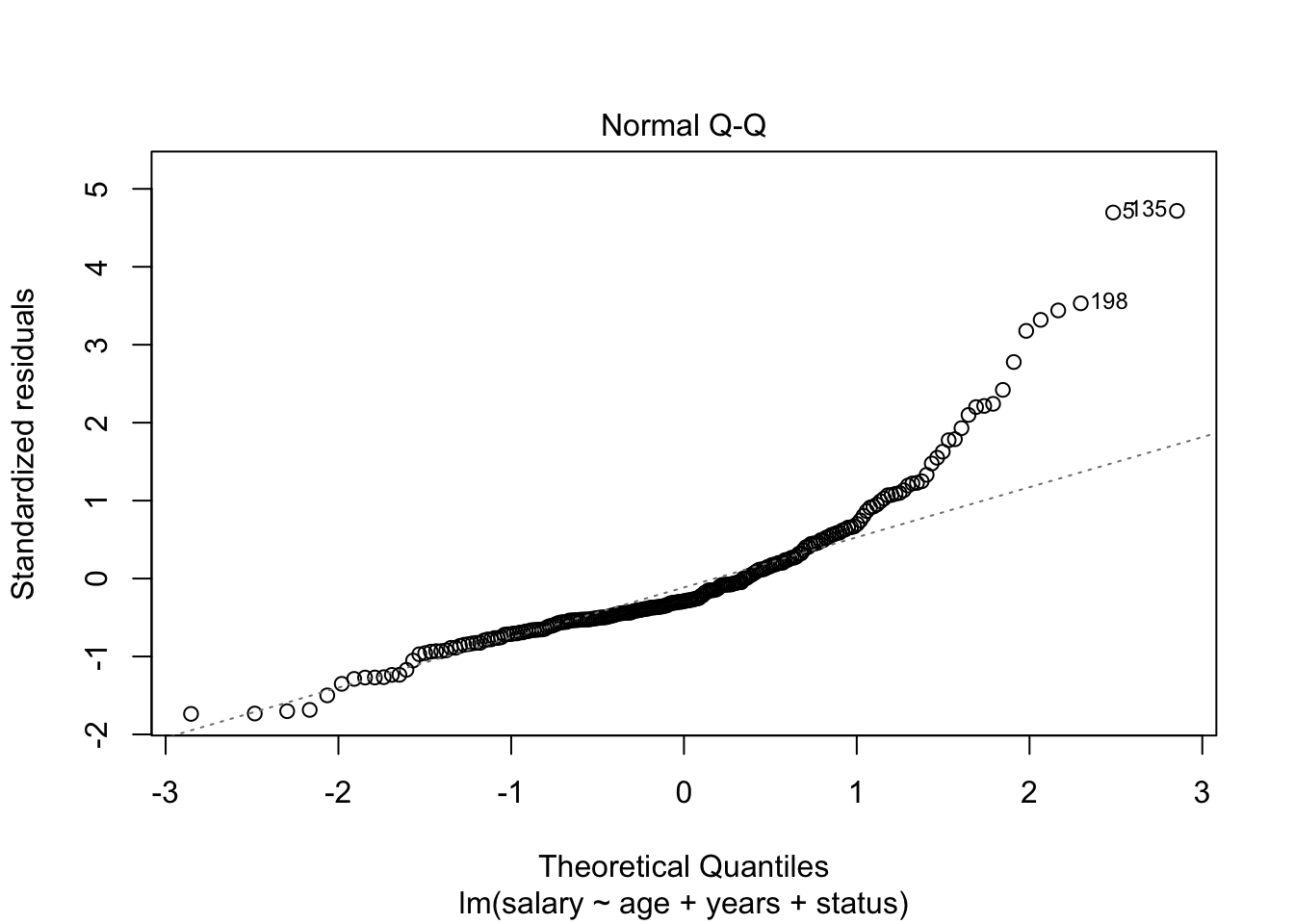
The normal Q-Q plot shows a highly non-normal distribution of residuals because the dashed line deviates considerably from the straight line (which indicates what you’d get from normally distributed errors).
Homoscedasticity and independence of errors
plot(model_lm, which = c(1, 3))
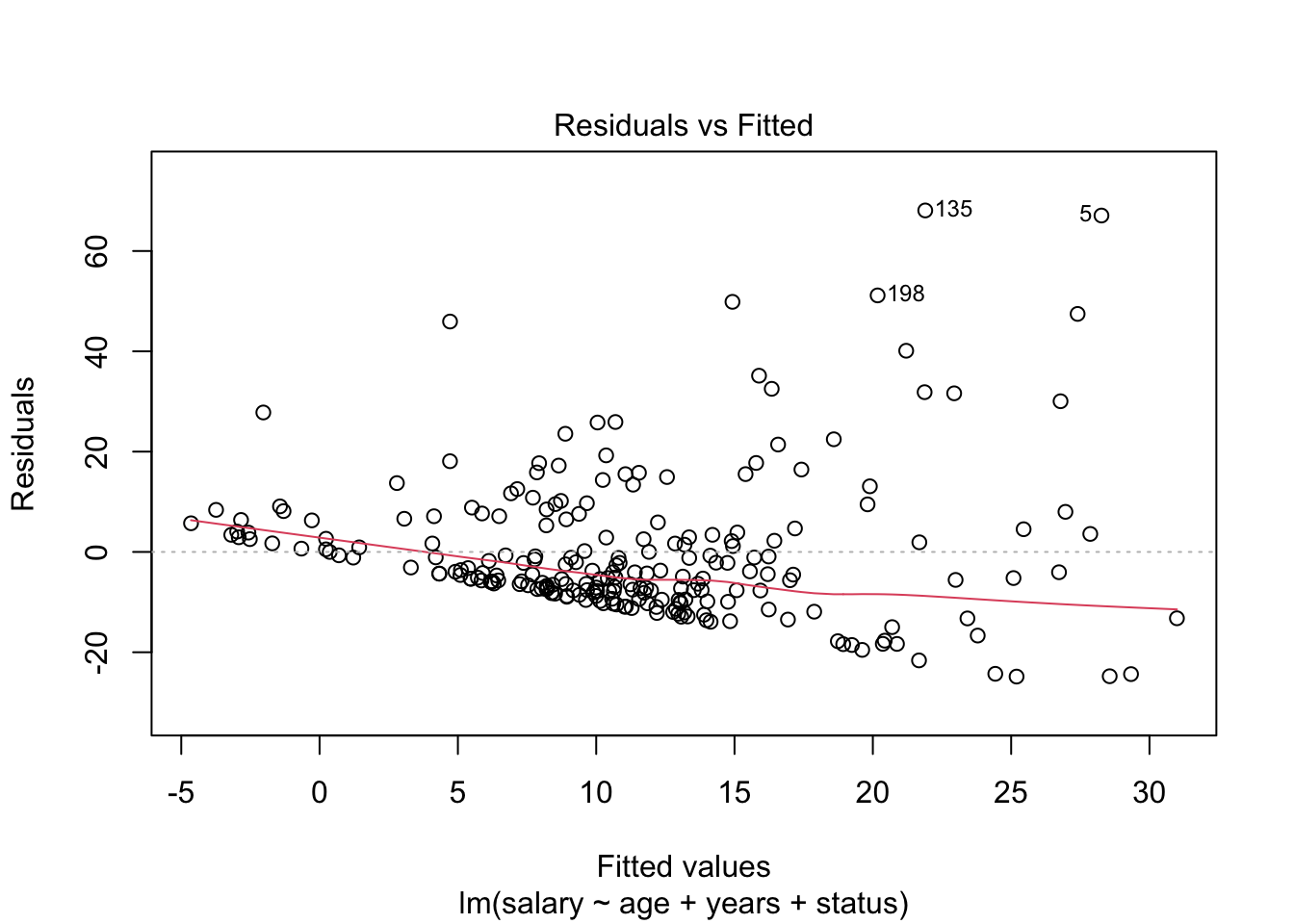
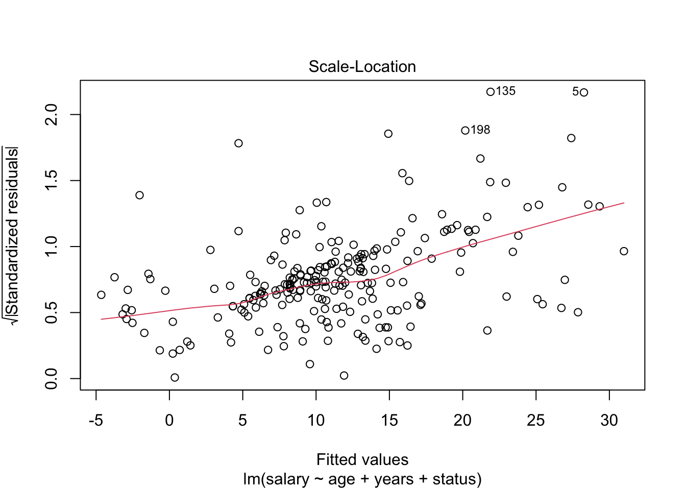
The scatterplots of fitted values vs residuals do not show a random pattern. There is a distinct funnelling, and the red trend line is not flat, indicating heteroscedasticity.
Multicollinearity
car::vif(model_lm)
##       age     years    status
## 12.652841 12.156757  1.153364
1/car::vif(model_lm)
##        age      years     status
## 0.07903364 0.08225878 0.86702902
car::vif(model_lm) %>%
  mean()
## [1] 8.65432
For the age and experience variables in the model, VIF values are above 10 (or alternatively, tolerance values are all well below 0.2), indicating multicollinearity in the data. In fact, the correlation between these two variables is around .9! So, these two variables are measuring very similar things. Of course, this makes perfect sense because the older a model is, the more years she would’ve spent modelling! So, it was fairly stupid to measure both of these things! This also explains the weird result that the number of years spent modelling negatively predicted salary (i.e. more experience = less salary!): in fact if you do a simple regression with experience as the only predictor of salary you’ll find it has the expected positive relationship. This hopefully demonstrates why multicollinearity can bias the regression model. All in all, several assumptions have not been met and so this model is probably fairly unreliable.
Task 8.5
A study was carried out to explore the relationship between aggression and several potential predicting factors in 666 children who had an older sibling. Variables measured were parenting_style (high score = bad parenting practices), computer_games (high score = more time spent playing computer games), television (high score = more time spent watching television), diet (high score = the child has a good diet low in harmful additives), and sibling_aggression (high score = more aggression seen in their older sibling). Past research indicated that parenting style and sibling aggression were good predictors of the level of aggression in the younger child. All other variables were treated in an exploratory fashion. Analyse them with a linear model (child_aggression.csv).
Load the data and fit the model. We need to conduct this analysis hierarchically, entering parenting_style and sibling_aggression in the first step (forced entry) and the remaining variables in a second step using a stepwise method (applying the step() function:
aggress_tib <- discovr::child_aggression

agress_lm <- lm(aggression ~ parenting_style + sibling_aggression, data = aggress_tib, na.action = na.exclude)
agress_full_lm <- update(agress_lm, .~. + television + computer_games + diet) %>%
  step()
## Start:  AIC=-1566.61
## aggression ~ parenting_style + sibling_aggression + television +
##     computer_games + diet
##
##                      Df Sum of Sq    RSS     AIC
## - television          1   0.04817 62.288 -1568.1
## <none>                            62.240 -1566.6
## - sibling_aggression  1   0.41840 62.658 -1564.2
## - diet                1   0.77357 63.014 -1560.4
## - computer_games      1   1.39822 63.638 -1553.8
## - parenting_style     1   1.42809 63.668 -1553.5
##
## Step:  AIC=-1568.1
## aggression ~ parenting_style + sibling_aggression + computer_games +
##     diet
##
##                      Df Sum of Sq    RSS     AIC
## <none>                            62.288 -1568.1
## - sibling_aggression  1   0.48054 62.769 -1565.0
## - diet                1   0.81815 63.106 -1561.4
## - computer_games      1   1.42689 63.715 -1555.0
## - parenting_style     1   2.28530 64.573 -1546.1
agress_full_lm %>%
  broom::glance() %>%
  knitr::kable(digits = 3)
| r.squared | adj.r.squared | sigma | statistic | p.value | df | logLik | AIC | BIC | deviance | df.residual | nobs |
|---|---|---|---|---|---|---|---|---|---|---|---|
| 0.082 | 0.076 | 0.307 | 14.735 | 0 | 4 | -155.963 | 323.927 | 350.935 | 62.288 | 661 | 666 |
agress_full_lm %>%
  broom::tidy() %>%
  knitr::kable(digits = 3)
| term | estimate | std.error | statistic | p.value |
|---|---|---|---|---|
| (Intercept) | -0.006 | 0.012 | -0.497 | 0.619 |
| parenting_style | 0.062 | 0.013 | 4.925 | 0.000 |
| sibling_aggression | 0.086 | 0.038 | 2.258 | 0.024 |
| computer_games | 0.143 | 0.037 | 3.891 | 0.000 |
| diet | -0.112 | 0.038 | -2.947 | 0.003 |
agress_full_lm %>%
  parameters::model_parameters(standardize = "refit", digits = 3) %>%
  knitr::kable()
| Parameter | Coefficient | SE | CI_low | CI_high | t | df_error | p |
|---|---|---|---|---|---|---|---|
| (Intercept) | 0.0000000 | 0.0372413 | -0.0731256 | 0.0731256 | 0.000000 | 661 | 1.0000000 |
| parenting_style | 0.1937732 | 0.0393481 | 0.1165109 | 0.2710356 | 4.924586 | 661 | 0.0000011 |
| sibling_aggression | 0.0883114 | 0.0391070 | 0.0115225 | 0.1651004 | 2.258198 | 661 | 0.0242586 |
| computer_games | 0.1534858 | 0.0394434 | 0.0760363 | 0.2309353 | 3.891291 | 661 | 0.0001098 |
| diet | -0.1177625 | 0.0399661 | -0.1962384 | -0.0392867 | -2.946560 | 661 | 0.0033264 |
agress_full_lm$anova
##           Step Df   Deviance Resid. Df Resid. Dev       AIC
## 1              NA         NA       660   62.23999 -1566.614
## 2 - television  1 0.04816702       661   62.28816 -1568.099
Based on the final model (which is actually all we’re interested in) the following variables predict aggression:
- Parenting style (b = 0.062, $ \beta $ = 0.194, t = 4.93, p < 0.001) significantly predicted aggression. The beta value indicates that as parenting increases (i.e. as bad practices increase), aggression increases also.
- Sibling aggression (b = 0.086, $ \beta $= 0.088, t = 2.26, p = 0.024) significantly predicted aggression. The beta value indicates that as sibling aggression increases (became more aggressive), aggression increases also.
- Computer games (b = 0.143, $ \beta $ = 0.037, t= 3.89, p < .001) significantly predicted aggression. The beta value indicates that as the time spent playing computer games increases, aggression increases also.
- Good diet (b = –0.112, $ \beta $ = –0.118, t = –2.95, p = 0.003) significantly predicted aggression. The beta value indicates that as the diet improved, aggression decreased.
The only factor not to predict aggression significantly was:
- Television did not predict aggression (base don the change in the AIC).
Based on the standardized beta values, the most substantive predictor of aggression was actually parenting style, followed by computer games, diet and then sibling aggression.
$ R^2 $ is the squared correlation between the observed values of aggression and the values of aggression predicted by the model, 8.2% of the variance in aggression is explained. With all four of these predictors in the model only 8.2% of the variance in aggression can be explained.
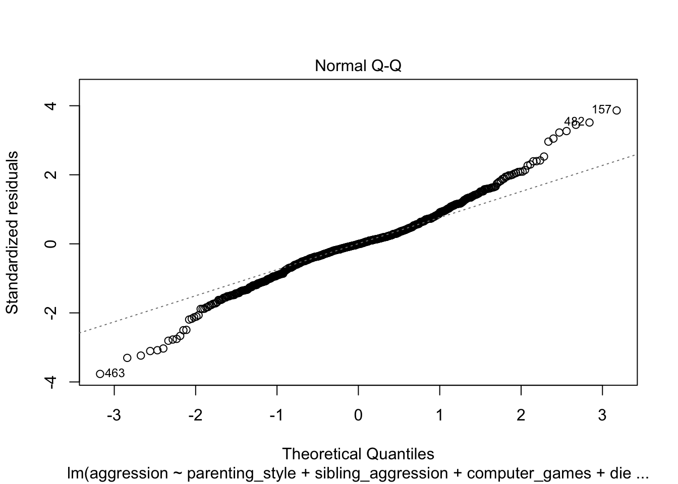
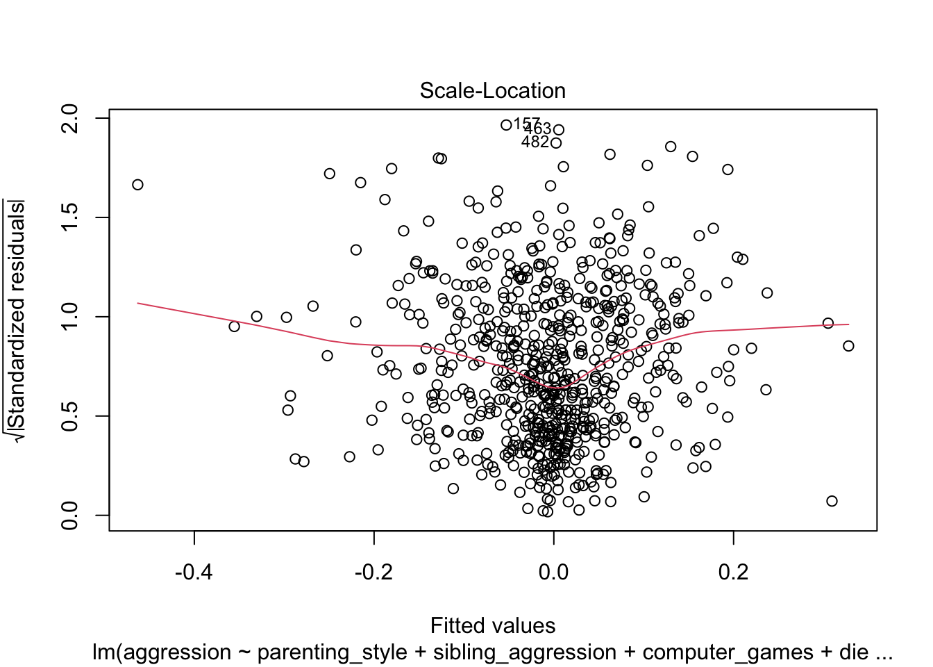
The Q-Q plot suggests that errors may well deviate from normally distributed:
plot(agress_full_lm, which = 2)
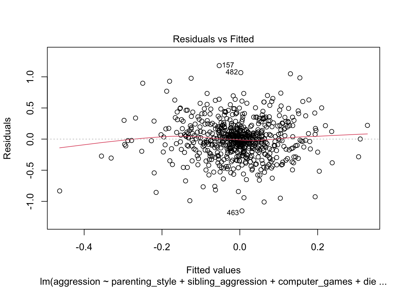
The scatterplot of predicted values vs residuals helps us to assess both homoscedasticity and independence of errors. The plot does show a random scatter, but the trend line is not completely flat. It would be useful to run a robust model.
plot(agress_full_lm, which = c(1, 3))
Using robust standard errors, sibling aggression is no longer significant.
agress_full_lm %>%
  parameters::model_parameters(robust = TRUE, vcov.type = "HC4") %>%
  knitr::kable(digits = 3)
| Parameter | Coefficient | SE | CI_low | CI_high | t | df_error | p |
|---|---|---|---|---|---|---|---|
| (Intercept) | -0.006 | 0.012 | -0.029 | 0.018 | -0.494 | 661 | 0.621 |
| parenting_style | 0.062 | 0.016 | 0.031 | 0.093 | 3.905 | 661 | 0.000 |
| sibling_aggression | 0.086 | 0.045 | -0.002 | 0.174 | 1.927 | 661 | 0.054 |
| computer_games | 0.143 | 0.048 | 0.050 | 0.237 | 3.019 | 661 | 0.003 |
| diet | -0.112 | 0.049 | -0.208 | -0.015 | -2.269 | 661 | 0.024 |
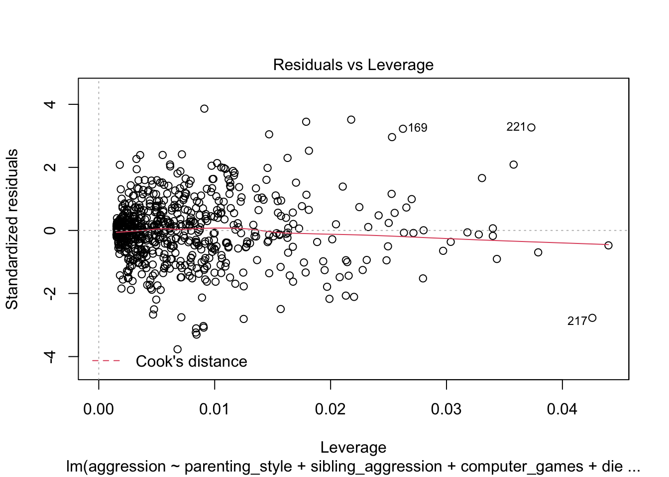
The influence plot looks fine. There are no extreme Cook’s distances and the trend line is fairly flat.
plot(agress_full_lm, which = 5)
Task 8.6
Repeat the analysis in Labcoat Leni’s Real Research 8.1 using bootstrapping for the confidence intervals. What are the confidence intervals for the regression parameters?
To recap, the models are fit as follows (see also the Labcoat Leni answers). Load the data directly from the discovr package:
ong_tib <- discovr::ong_2011
Fit the models that look at whether narcissism predicts, above and beyond the other variables, the frequency of status updates.
# Fit the models
ong_base_lm <- lm(status ~ sex + age + grade, data = ong_tib, na.action = na.exclude)
ong_ext_lm <- update(ong_base_lm, .~. + extraversion)
ong_ncs_lm <- update(ong_ext_lm, .~. + narcissism)

# Compare models
anova(ong_base_lm, ong_ext_lm, ong_ncs_lm) %>%
  broom::tidy() %>%
  knitr::kable(digits = 3)
| res.df | rss | df | sumsq | statistic | p.value |
|---|---|---|---|---|---|
| 246 | 1481.515 | NA | NA | NA | NA |
| 245 | 1458.360 | 1 | 23.155 | 4.017 | 0.046 |
| 244 | 1406.600 | 1 | 51.759 | 8.979 | 0.003 |
Fit the models that look at whether narcissism predicts, above and beyond the other variables, the Facebook profile picture ratings.
# Fit models
prof_base_lm <- lm(profile ~ sex + age + grade, data = ong_tib, na.action = na.exclude)
prof_ext_lm <- update(prof_base_lm, .~. + extraversion)
prof_ncs_lm <- update(prof_ext_lm, .~. + narcissism)

# Compare models

anova(prof_base_lm, prof_ext_lm, prof_ncs_lm) %>%
  broom::tidy()  %>%
  knitr::kable(digits = 3)
| res.df | rss | df | sumsq | statistic | p.value |
|---|---|---|---|---|---|
| 188 | 2405.233 | NA | NA | NA | NA |
| 187 | 2104.969 | 1 | 300.264 | 29.613 | 0 |
| 186 | 1885.958 | 1 | 219.011 | 21.600 | 0 |
Facebook status update frequency
Get the bootstrap CIs:
ong_ncs_lm %>%
  parameters::model_parameters(bootstrap = TRUE, digits = 3) %>%
  knitr::kable(digits = 3)
| Parameter | Coefficient | CI_low | CI_high | p |
|---|---|---|---|---|
| (Intercept) | 0.136 | -5.152 | 5.158 | 0.943 |
| sexMale | -0.947 | -1.572 | -0.363 | 0.004 |
| age | -0.012 | -0.341 | 0.363 | 0.933 |
| gradeSec 2 | -0.432 | -1.280 | 0.505 | 0.348 |
| gradeSec 3 | -1.006 | -2.101 | -0.001 | 0.050 |
| extraversion | 0.010 | -0.049 | 0.063 | 0.735 |
| narcissism | 0.067 | 0.025 | 0.107 | 0.004 |
The main benefit of the bootstrap confidence intervals and significance values is that they do not rely on assumptions of normality or homoscedasticity, so they give us an accurate estimate of the true population value of b for each predictor. The bootstrapped confidence intervals in the output do not affect the conclusions reported in Ong et al. (2011). Ong et al.’s prediction was still supported in that, after controlling for age, grade and sex, narcissism significantly predicted the frequency of Facebook status updates over and above extroversion, b = 0.066 [0.03, 0.10], p < 0.001.
Facebook profile picture rating
Get the bootstrap CIs:
prof_ncs_lm %>%
  parameters::model_parameters(bootstrap = TRUE) %>%
  knitr::kable(digits = 3)
| Parameter | Coefficient | CI_low | CI_high | p |
|---|---|---|---|---|
| (Intercept) | -3.843 | -18.934 | 8.564 | 0.563 |
| sexMale | 0.568 | -0.539 | 1.650 | 0.344 |
| age | 0.348 | -0.541 | 1.425 | 0.426 |
| gradeSec 2 | -0.522 | -2.163 | 0.920 | 0.501 |
| gradeSec 3 | -0.634 | -3.056 | 1.364 | 0.567 |
| extraversion | 0.109 | 0.023 | 0.203 | 0.006 |
| narcissism | 0.173 | 0.104 | 0.242 | 0.000 |
Similarly, the bootstrapped confidence intervals for the second regression are consistent with the conclusions reported in Ong et al. (2011). That is, after adjusting for age, grade and sex, narcissism significantly predicted the Facebook profile picture ratings over and above extroversion, b = 0.171 [0.10, 0.24], p < 0.001.
Task 8.7
Coldwell, Pike and Dunn (2006) investigated whether household chaos predicted children’s problem behaviour over and above parenting. From 118 families they recorded the age and gender of the youngest child (child_age and child_gender). They measured dimensions of the child’s perceived relationship with their mum: (1) warmth/enjoyment (child_warmth), and (2) anger/hostility (child_anger). Higher scores indicate more warmth/enjoyment and anger/hostility respectively. They measured the mum’s perceived relationship with her child, resulting in dimensions of positivity (mum_pos) and negativity (mum_neg). Household chaos (chaos) was assessed. The outcome variable was the child’s adjustment (sdq): the higher the score, the more problem behaviour the child was reported to be displaying. Conduct a hierarchical linear model in three steps: (1) enter child age and gender; (2) add the variables measuring parent-child positivity, parent-child negativity, parent-child warmth, parent-child anger; (3) add chaos. Is household chaos predictive of children’s problem behaviour over and above parenting? (coldwell_2006.csv).
Load the data:
chaos_tib <- discovr::coldwell_2006
Write a function to round values in the output!
round_values <- function(tibble, digits = 3){
  require(dplyr)
  tibble <- tibble %>%
  dplyr::mutate(
    dplyr::across(where(is.numeric), ~round(., 3))
  )
  return(tibble)
}
Model 1: sdq predicted from child_age and child_gender:
chaos_base_lm <- lm(sdq ~ child_age + child_age, data = chaos_tib, na.action = na.exclude)

chaos_base_lm %>%
  broom::glance() %>%
  round_values() %>%
  knitr::kable()
| r.squared | adj.r.squared | sigma | statistic | p.value | df | logLik | AIC | BIC | deviance | df.residual | nobs |
|---|---|---|---|---|---|---|---|---|---|---|---|
| 0.001 | -0.009 | 0.172 | 0.095 | 0.759 | 1 | 37.285 | -68.569 | -60.551 | 3.121 | 105 | 107 |
chaos_base_lm %>%
  broom::tidy() %>%
  round_values() %>%
  knitr::kable()
| term | estimate | std.error | statistic | p.value |
|---|---|---|---|---|
| (Intercept) | 1.247 | 0.144 | 8.642 | 0.000 |
| child_age | 0.001 | 0.002 | 0.308 | 0.759 |
Model 2: In a new block, add child_anger, child_warmth, mum_pos and mum_neg into the model:
chaos_emo_lm <- update(chaos_base_lm, .~. + child_anger + child_warmth + mum_pos + mum_neg)
chaos_emo_lm %>%
  broom::glance() %>%
  round_values() %>%
  knitr::kable()
| r.squared | adj.r.squared | sigma | statistic | p.value | df | logLik | AIC | BIC | deviance | df.residual | nobs |
|---|---|---|---|---|---|---|---|---|---|---|---|
| 0.061 | 0.008 | 0.174 | 1.159 | 0.335 | 5 | 34.65 | -55.301 | -37.35 | 2.731 | 90 | 96 |
chaos_emo_lm %>%
  broom::tidy() %>%
  round_values() %>%
  knitr::kable()
| term | estimate | std.error | statistic | p.value |
|---|---|---|---|---|
| (Intercept) | 0.943 | 0.332 | 2.843 | 0.006 |
| child_age | 0.001 | 0.002 | 0.590 | 0.556 |
| child_anger | 0.007 | 0.017 | 0.381 | 0.704 |
| child_warmth | -0.008 | 0.025 | -0.340 | 0.735 |
| mum_pos | 0.003 | 0.005 | 0.529 | 0.598 |
| mum_neg | 0.013 | 0.006 | 2.158 | 0.034 |
Model 3: In a final block, add chaos to the model:
chaos_chaos_lm <- update(chaos_emo_lm, .~. + chaos)
chaos_chaos_lm %>%
  broom::glance() %>%
  round_values() %>%
  knitr::kable()
| r.squared | adj.r.squared | sigma | statistic | p.value | df | logLik | AIC | BIC | deviance | df.residual | nobs |
|---|---|---|---|---|---|---|---|---|---|---|---|
| 0.104 | 0.044 | 0.171 | 1.725 | 0.124 | 6 | 36.934 | -57.867 | -37.352 | 2.604 | 89 | 96 |
chaos_chaos_lm %>%
  broom::tidy() %>%
  round_values() %>%
  knitr::kable()
| term | estimate | std.error | statistic | p.value |
|---|---|---|---|---|
| (Intercept) | 0.763 | 0.337 | 2.266 | 0.026 |
| child_age | 0.002 | 0.002 | 0.656 | 0.514 |
| child_anger | 0.003 | 0.017 | 0.190 | 0.850 |
| child_warmth | -0.002 | 0.025 | -0.093 | 0.926 |
| mum_pos | 0.003 | 0.005 | 0.507 | 0.613 |
| mum_neg | 0.011 | 0.006 | 1.859 | 0.066 |
| chaos | 0.074 | 0.036 | 2.082 | 0.040 |
chaos_chaos_lm %>%
  parameters::model_parameters(standardize = "refit", digits = 3) %>%
  knitr::kable()
| Parameter | Coefficient | SE | CI_low | CI_high | t | df_error | p |
|---|---|---|---|---|---|---|---|
| (Intercept) | 0.0000000 | 0.0998042 | -0.1983088 | 0.1983088 | 0.0000000 | 89 | 1.0000000 |
| child_age | 0.0675926 | 0.1030422 | -0.1371501 | 0.2723353 | 0.6559696 | 89 | 0.5135360 |
| child_anger | 0.0198999 | 0.1047546 | -0.1882453 | 0.2280451 | 0.1899668 | 89 | 0.8497677 |
| child_warmth | -0.0101373 | 0.1088309 | -0.2263818 | 0.2061073 | -0.0931469 | 89 | 0.9259962 |
| mum_pos | 0.0523631 | 0.1032264 | -0.1527456 | 0.2574718 | 0.5072645 | 89 | 0.6132239 |
| mum_neg | 0.1988785 | 0.1070043 | -0.0137368 | 0.4114939 | 1.8586029 | 89 | 0.0663887 |
| chaos | 0.2163831 | 0.1039170 | 0.0099023 | 0.4228639 | 2.0822697 | 89 | 0.0401883 |
We can’t compare the models because they’re based on different amounts of data (missing values)
From the output we can conclude that household chaos significantly predicted younger sibling’s problem behaviour over and above maternal parenting, child age and gender, t(88) = 2.08, p = 0.040. The positive standardized beta value (0.216) indicates that there is a positive relationship between household chaos and child’s problem behaviour. In other words, the higher the level of household chaos, the more problem behaviours the child displayed. The value of \(R^2\) (0.10) tells us that household chaos accounts for 10% of the variance in child problem behaviour.