Smart Alex solutions Chapter 7
This document contains abridged sections from Discovering Statistics Using R and RStudio by Andy Field so there are some copyright considerations. You can use this material for teaching and non-profit activities but please do not meddle with it or claim it as your own work. See the full license terms at the bottom of the page.
Task 7.1
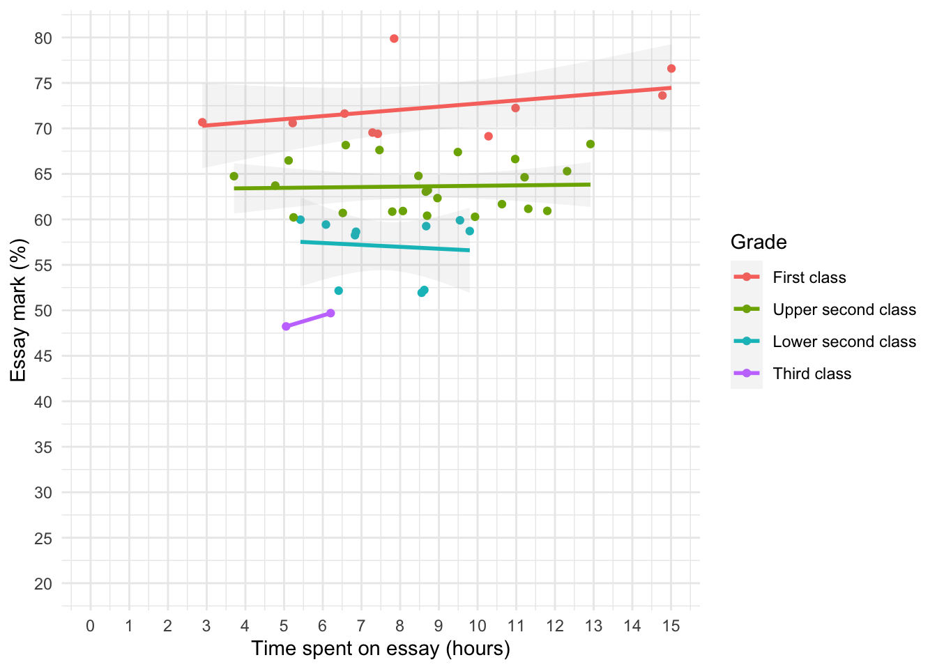
A student was interested in whether there was a positive relationship between the time spent doing an essay and the mark received. He got 45 of his friends and timed how long they spent writing an essay (hours) and the percentage they got in the essay (essay). He also translated these grades into their degree classifications (grade): in the UK, a student can get a first-class mark (the best), an upper-second-class mark, a lower second, a third, a pass or a fail (the worst). Using the data in the file essay_marks.csv find out what the relationship was between the time spent doing an essay and the eventual mark in terms of percentage and degree class (draw a scatterplot too).
Load the data
essay_tib <- readr::read_csv("../data/essay_marks.csv") %>%
  dplyr::mutate(
    grade = forcats::as_factor(grade)
  )
Alternative, load the data directly from the discovr package:
essay_tib <- discovr::essay_marks
Visualise the data
We’re interested in looking at the relationship between hours spent on an essay and the grade obtained. We could create a scatterplot of hours spent on the essay (x-axis) and essay mark (y-axis). I’ve chosen to highlight the degree classification grades using different colours.
ggplot2::ggplot(essay_tib, aes(hours, essay, colour = grade)) +
  geom_point() +
  geom_smooth(method = "lm", alpha = 0.1) +
  coord_cartesian(xlim = c(0, 15), ylim = c(20, 80)) +
  scale_x_continuous(breaks = seq(0, 15, 1)) +
  scale_y_continuous(breaks = seq(20, 80, 5)) +
  labs(x = "Time spent on essay (hours)", y = "Essay mark (%)", colour = "Grade", fill = "Grade") +
  theme_minimal()
Correlations
essay_tib %>%
  dplyr::select(hours, essay) %>%
  correlation::correlation() %>%
  knitr::kable(digits = 3)
| Parameter1 | Parameter2 | r | CI_low | CI_high | t | df | p | Method | n_Obs |
|---|---|---|---|---|---|---|---|---|---|
| hours | essay | 0.267 | -0.029 | 0.52 | 1.814 | 43 | 0.077 | Pearson | 45 |
The results in the table above indicate that the relationship between time spent writing an essay and grade awarded was not significant, Pearson’s r = 0.27, p = 0.077.
The second part of the question asks us to do the same analysis but when the percentages are recoded into degree classifications. The degree classifications are ordinal data (not interval): they are ordered categories. So we shouldn’t use Pearson’s test statistic, but Spearman’s and Kendall’s ones instead. Grade is a factor:
essay_tib$grade
##  [1] Upper second class First class        Third class        First class
##  [5] Lower second class Upper second class Upper second class Upper second class
##  [9] Upper second class Third class        Upper second class First class
## [13] First class        Lower second class Lower second class Upper second class
## [17] Upper second class Upper second class Upper second class Lower second class
## [21] Lower second class First class        Upper second class Upper second class
## [25] First class        Upper second class Lower second class Lower second class
## [29] Lower second class First class        Upper second class Upper second class
## [33] Upper second class First class        First class        Upper second class
## [37] Upper second class Upper second class Upper second class Upper second class
## [41] Upper second class Upper second class Lower second class Lower second class
## [45] First class
## Levels: First class Upper second class Lower second class Third class
We need to convert it into numbers using as.numeric:
essay_tib <- essay_tib %>%
  dplyr::mutate(
    grade_num = as.numeric(grade)
    )
Let’s check the numeric grade matches the description (i.e. first = 1, upper second = 2 etc.):
| id | essay | hours | grade | grade_num |
|---|---|---|---|---|
| qxbcjg | 61.68 | 10.63 | Upper second class | 2 |
| csykgu | 69.55 | 7.29 | First class | 1 |
| npxgpl | 48.23 | 5.05 | Third class | 4 |
| gomiwl | 70.68 | 2.89 | First class | 1 |
| qdywaa | 59.90 | 9.55 | Lower second class | 3 |
| cmaprb | 61.16 | 11.31 | Upper second class | 2 |
| nrvhix | 67.62 | 7.47 | Upper second class | 2 |
| ybytlf | 64.78 | 8.47 | Upper second class | 2 |
| talwvg | 63.21 | 8.72 | Upper second class | 2 |
| ceylea | 49.69 | 6.20 | Third class | 4 |
| berjky | 63.72 | 4.77 | Upper second class | 2 |
| cjxgpl | 72.24 | 10.98 | First class | 1 |
| gufenh | 70.59 | 5.22 | First class | 1 |
| uaxxdm | 58.64 | 6.86 | Lower second class | 3 |
| unnhpl | 58.72 | 9.80 | Lower second class | 3 |
Now the correlation:
essay_tib %>%
  dplyr::select(hours, grade_num) %>%
  correlation::correlation(method = "spearman") %>%
  knitr::kable(digits = 3)
| Parameter1 | Parameter2 | rho | CI_low | CI_high | S | p | Method | n_Obs |
|---|---|---|---|---|---|---|---|---|
| hours | grade_num | -0.193 | -0.461 | 0.106 | 18110.93 | 0.204 | Spearman | 45 |
There was no significant relationship between degree grade classification for an essay and the time spent doing it, $ \rho_s = -0.19 $, p = 0.204. Note that the direction of the relationship has reversed. This has happened because the essay marks were recoded as 1 (first), 2 (upper second), 3 (lower second), and 4 (third), so high grades were represented by low numbers.
Task 7.2
Using the notebook.csv data from Chapter 3, find out if the size of relationship between the participant’s sex and arousal.
Load the data
library(tidyverse)
notebook_tib <- readr::read_csv("../data/essay_marks.csv") %>%
  dplyr::mutate(
    sex = forcats::as_factor(sex),
    film = forcats::as_factor(film)
  )
Alternative, load the data directly from the discovr package:
notebook_tib <- discovr::notebook
Estimate the correlation
Sex is a categorical variable with two categories, therefore, we need to quantify this relationship using a point-biserial correlation.
notebook_tib %>%
  dplyr::mutate(
    sex_bin = ifelse(sex == "Male", 0, 1),
  ) %>%
  dplyr::select(arousal, sex_bin) %>%
  correlation::correlation() %>%
  knitr::kable(digits = 3)
| Parameter1 | Parameter2 | r | CI_low | CI_high | t | df | p | Method | n_Obs |
|---|---|---|---|---|---|---|---|---|---|
| arousal | sex_bin | -0.196 | -0.478 | 0.123 | -1.232 | 38 | 0.226 | Pearson | 40 |
I used a two-tailed test because one-tailed tests should never really be used. There was no significant relationship between biological sex and arousal because the p-value is larger than 0.05, \(r_\text{pb}\) = –0.20, p = 0.226.
Task 7.3
Using the notebook data again, quantify the relationship between the film watched and arousal.
notebook_tib %>%
  dplyr::mutate(
    film_bin = ifelse(film == "The notebook", 0, 1),
  ) %>%
  dplyr::select(arousal, film_bin) %>%
  correlation::correlation() %>%
  knitr::kable(digits = 3)
| Parameter1 | Parameter2 | r | CI_low | CI_high | t | df | p | Method | n_Obs |
|---|---|---|---|---|---|---|---|---|---|
| arousal | film_bin | -0.865 | -0.927 | -0.757 | -10.606 | 38 | 0 | Pearson | 40 |
There was a significant relationship between the film watched and arousal, \(r_\text{pb}\) = –0.86, p < 0.001. Looking at how the groups were coded, you should see that The Notebook had a code of 0, and the documentary about notebooks had a code of 1, therefore the negative coefficient reflects the fact that as film goes up (changes from 0 to 1) arousal goes down. Put another way, as the film changes from The Notebook to a documentary about notebooks, arousal decreases. So The Notebook gave rise to the greater arousal levels.
Task 7.4
As a statistics lecturer I am interested in the factors that determine whether a student will do well on a statistics course. Imagine I took 25 students and looked at their grades for my statistics course at the end of their first year at university: first, upper second, lower second and third class (see Task 1). I also asked these students what grade they got in their high school maths exams. In the UK GCSEs are school exams taken at age 16 that are graded A, B, C, D, E or F (an A grade is the best). The data for this study are in the file grades.csv. To what degree does GCSE maths grade correlate with first-year statistics grade?
Load the data
The categories in the data file have a meaningful order, so after importing the data we transform stats and gcse to factors but also order the factor levels in the correct order (this is important!).
grade_tib <- readr::read_csv("../data/grades.csv") %>%
  dplyr::mutate(
    stats = forcats::as_factor(stats) %>% forcats::fct_relevel("First class", "Upper second class", "Lower second class", "Third class", "Pass", "Fail"),
    gcse = forcats::as_factor(gcse) %>% forcats::fct_relevel("A", "B", "C", "D", "E", "F")
  )
Alternative, load the data directly from the discovr package:
grade_tib <- discovr::grades
Estimate the correlation
Let’s look at these variables. In the UK, GCSEs are school exams taken at age 16 that are graded A, B, C, D, E or F. These grades are categories that have an order of importance (an A grade is better than all of the lower grades). In the UK, a university student can get a first-class mark, an upper second, a lower second, a third, a pass or a fail. These grades are categories, but they have an order to them (an upper second is better than a lower second). When you have categories like these that can be ordered in a meaningful way, the data are said to be ordinal. The data are not interval, because a first-class degree encompasses a 30% range (70–100%), whereas an upper second only covers a 10% range (60–70%). When data have been measured at only the ordinal level they are said to be non-parametric and Pearson’s correlation is not appropriate. Therefore, the Spearman correlation coefficient is used.
In the file, the scores are in two columns: one labelled stats and one labelled gcse.
Table: Table 1: First 10 rows of grade_tib
| id | stats | gcse |
|---|---|---|
| wbmew | First class | A |
| ypusy | First class | A |
| sbumv | First class | C |
| wqicp | Upper second class | C |
| xnobi | Upper second class | C |
| glxdw | Upper second class | D |
| eomcn | Upper second class | E |
| bjhcl | Lower second class | A |
| wcype | Lower second class | B |
| grkvu | Lower second class | C |
The first thing we need to do is to convert stats and gcse to numbers using as.numeric, which will return the numeric value attached to each factor level:
grade_tib <- grade_tib %>%
  dplyr::mutate(
    stat_num = as.numeric(stats),
    gcse_num = as.numeric(gcse)
    )
Let’s check the numeric grade matches the description (i.e. first = 1, upper second = 2 etc.):
Table: Table 2: First 10 rows of grade_tib
| id | stats | gcse | stat_num | gcse_num |
|---|---|---|---|---|
| wbmew | First class | A | 1 | 1 |
| ypusy | First class | A | 1 | 1 |
| sbumv | First class | C | 1 | 3 |
| wqicp | Upper second class | C | 2 | 3 |
| xnobi | Upper second class | C | 2 | 3 |
| glxdw | Upper second class | D | 2 | 4 |
| eomcn | Upper second class | E | 2 | 5 |
| bjhcl | Lower second class | A | 3 | 1 |
| wcype | Lower second class | B | 3 | 2 |
| grkvu | Lower second class | C | 3 | 3 |
Now the correlation:
grade_tib %>%
  dplyr::select(stat_num, gcse_num) %>%
  correlation::correlation(method = "spearman") %>%
  knitr::kable(digits = 3)
| Parameter1 | Parameter2 | rho | CI_low | CI_high | S | p | Method | n_Obs |
|---|---|---|---|---|---|---|---|---|
| stat_num | gcse_num | 0.455 | 0.072 | 0.72 | 1418.035 | 0.022 | Spearman | 25 |
In the question I predicted that better grades in GCSE maths would correlate with better degree grades for my statistics course. This hypothesis is directional and so a one-tailed test could be selected; however, in the chapter I advised against one-tailed tests so I have done two-tailed.
We could report these results as follows:
- There was a significant positive relationship between a person’s statistics grade and their GCSE maths grade, $ r_\text{s} $ = 0.45, *p* = 0.022.
Task 7.5
In Figure 3.4 we saw some data relating to people’s ratings of dishonest acts and the likeableness of the perpetrator (for a full description see Jane Superbrain Box 3.1). Compute the Spearman correlation between ratings of dishonesty and likeableness of the perpetrator. The data are in honesty_lab.csv.
Load the data
honesty_tib <- readr::read_csv("../data/honesty_lab.csv") %>%
  dplyr::mutate(
    sex = forcats::as_factor(sex),
    film = forcats::as_factor(film)
  )
Alternative, load the data directly from the discovr package:
honesty_tib <- discovr::honesty_lab
Estimate the correlation
honesty_tib %>%
  dplyr::select(deed, likeableness) %>%
  correlation::correlation(method = "spearman") %>%
  knitr::kable(digits = 3)
| Parameter1 | Parameter2 | rho | CI_low | CI_high | S | p | Method | n_Obs |
|---|---|---|---|---|---|---|---|---|
| deed | likeableness | 0.844 | 0.776 | 0.892 | 26054.24 | 0 | Spearman | 100 |
The relationship between ratings of dishonesty and likeableness of the perpetrator was significant because the p-value is less than 0.05 (p = 0.000). The value of Spearman’s correlation coefficient is quite large and positive (0.84), indicating a large positive effect: the more likeable the perpetrator was, the more positively their dishonest acts were viewed.
We could report the results as follows:
- There was a large and significant positive relationship between the likeableness of a perpetrator and how positively their dishonest acts were viewed,
\(r_\text{s}\)= 0.84, p < 0.001.
Task 7.6
In Chapter 1 (Task 6) we looked at data from people who had been forced to marry goats and dogs and measured their life satisfaction and, also, how much they like animals (goat_or_dog.csv). Is there a significant correlation between life satisfaction and the type of animal to which a person was married
Load the data
goat_tib <- readr::read_csv("../data/goat_or_dog.csv") %>%
  dplyr::mutate(
    wife = forcats::as_factor(wife)
  )
Alternative, load the data directly from the discovr package:
goat_tib <- discovr::animal_bride
Estimate the correlation
Wife is a categorical variable with two categories (goat or dog). Therefore, we need to look at this relationship using a point-biserial correlation.
goat_tib <- goat_tib %>%
  dplyr::mutate(
    wife_bin = ifelse(wife == "Goat", 0, 1),
  )

goat_tib %>%
  dplyr::select(life_satisfaction, wife_bin) %>%
  correlation::correlation() %>%
  knitr::kable(digits = 3)
| Parameter1 | Parameter2 | r | CI_low | CI_high | t | df | p | Method | n_Obs |
|---|---|---|---|---|---|---|---|---|---|
| life_satisfaction | wife_bin | 0.63 | 0.261 | 0.839 | 3.446 | 18 | 0.003 | Pearson | 20 |
I used a two-tailed test because one-tailed tests should never really be used (see book chapter for more explanation). As you can see there, was a significant relationship between type of animal wife and life satisfaction because our p-value is less than 0.05, \(r_\text{pb}\) = 0.63, p = 0.003. Looking at how the groups were coded, you should see that goat had a code of 0 and dog had a code of 1, therefore this result reflects the fact that as wife goes up (changes from 0 to 1) life satisfaction goes up. Put another way, as wife changes from goat to dog, life satisfaction increases. So, being married to a dog was associated with greater life satisfaction.
Task 7.7
Repeat the analysis above taking account of animal liking when computing the correlation between life satisfaction and the animal to which a person was married.
We can conduct a partial correlation between life satisfaction and the animal to which a person was married while ‘adjusting’ for the effect of liking animals. Remember that we added the variable wife_bin to goat_tib in the previous solution.
goat_tib %>%
  dplyr::select(-wife) %>%
  correlation::correlation(partial = TRUE) %>%
  knitr::kable(digits = 3)
| Parameter1 | Parameter2 | r | CI_low | CI_high | t | df | p | Method | n_Obs |
|---|---|---|---|---|---|---|---|---|---|
| animal | life_satisfaction | 0.615 | 0.236 | 0.831 | 3.306 | 18 | 0.008 | Pearson | 20 |
| animal | wife_bin | -0.399 | -0.715 | 0.053 | -1.846 | 18 | 0.081 | Pearson | 20 |
| life_satisfaction | wife_bin | 0.701 | 0.375 | 0.873 | 4.173 | 18 | 0.002 | Pearson | 20 |
Notice that the partial correlation between wife and life satisfaction is 0.70, which is greater than the correlation when the effect of animal liking is not adjusted for (r = 0.630 from the previous task). The correlation has become more statistically significant (its p-value has decreased from 0.003 to 0.002..)
Running this analysis has shown us that type of wife alone explains a large portion of the variation in life satisfaction. In other words, the relationship between wife and life satisfaction is not due to animal liking.
Task 7.8
In Chapter 1 (Task 7) we looked at data based on findings that the number of cups of tea drunk was related to cognitive functioning (Feng et al., 2010). The data are in the file tea_makes_you_brainy_15.csv. What is the correlation between tea drinking and cognitive functioning? Is there a significant effect?
Load the data
tea15_tib <- readr::read_csv("../data/tea_makes_you_brainy_15.csv")
Alternative, load the data directly from the discovr package:
tea15_tib <- discovr::tea_15
Estimate the correlation
Because the numbers of cups of tea and cognitive function are both interval variables, we can conduct a Pearson’s correlation coefficient.
tea15_tib %>%
  dplyr::select(tea, cog_fun) %>%
  correlation::correlation() %>%
  knitr::kable(digits = 3)
| Parameter1 | Parameter2 | r | CI_low | CI_high | t | df | p | Method | n_Obs |
|---|---|---|---|---|---|---|---|---|---|
| tea | cog_fun | 0.078 | -0.453 | 0.567 | 0.281 | 13 | 0.783 | Pearson | 15 |
I chose a two-tailed test because it is never really appropriate to conduct a one-tailed test (see the book chapter). The results in the table above indicate that the relationship between number of cups of tea drunk per day and cognitive function was not significant. We can tell this because our p-value is greater than 0.05. Pearson’s r = 0.08, p = 0.783.
Task 7.9
The research in the previous task was replicated but in a larger sample (N = 716), which is the same as the sample size in Feng et al.’s research (tea_makes_you_brainy_716.csv). Conduct a correlation between tea drinking and cognitive functioning. Compare the correlation coefficient and significance in this large sample, with the previous task. What statistical point do the results illustrate?
Load the data
tea716_tib <- readr::read_csv("../data/tea_makes_you_brainy_716.csv")
Alternative, load the data directly from the discovr package:
tea716_tib <- discovr::tea_716
Estimate the correlation
tea716_tib %>%
  dplyr::select(tea, cog_fun) %>%
  correlation::correlation() %>%
  knitr::kable(digits = 3)
| Parameter1 | Parameter2 | r | CI_low | CI_high | t | df | p | Method | n_Obs |
|---|---|---|---|---|---|---|---|---|---|
| tea | cog_fun | 0.078 | 0.004 | 0.15 | 2.081 | 714 | 0.038 | Pearson | 716 |
We can see that although the value of Pearson’s r has not changed, it is still very small (0.08), the relationship between the number of cups of tea drunk per day and cognitive function is now just significant (p = 0.038). This example indicates one of the downfalls of significance testing; you can get significant results when you have large sample sizes even if the effect is very small. Basically, whether you get a significant result or not is entirely subject to the sample size.
Task 7.10
In Chapter 6 we looked at hygiene scores over three days of a rock music festival (download_festival.csv). Using Spearman’s correlation, were hygiene scores on day 1 of the festival significantly correlated with those on day 3?
Load the data
download_tib <- readr::read_csv("../data/download_festival.csv") %>%
  dplyr::mutate(
    gender = forcats::as_factor(gender)
  )
Alternative, load the data directly from the discovr package:
download_tib <- discovr::download
Estimate the correlation
First, we need to make the data messy so that scores for different days are in different columns (rather than different rows):
download_tib %>%
  dplyr::select(day_1, day_3) %>%
  correlation::correlation(method = "spearman") %>%
  knitr::kable(digits = 3)
| Parameter1 | Parameter2 | rho | CI_low | CI_high | S | p | Method | n_Obs |
|---|---|---|---|---|---|---|---|---|
| day_1 | day_3 | 0.344 | 0.178 | 0.491 | 203307.3 | 0 | Spearman | 123 |
The hygiene scores on day 1 of the festival correlated significantly with hygiene scores on day 3. The value of Spearman’s correlation coefficient is 0.344, which is a positive value suggesting that the smellier you are on day 1, the smellier you will be on day 3, \(r_\text{s}\) = 0.34, p < 0.001.
Task 7.11
Using the data in shopping_exercise.csv (Chapter 1, Task 5), find out if there is a significant relationship between the time spent shopping and the distance covered.
Load the data
shopping_tib <- readr::read_csv("../data/shopping_exercise.csv") %>%
  dplyr::mutate(
    sex = forcats::as_factor(sex)
  )
Alternative, load the data directly from the discovr package:
shopping_tib <- discovr::shopping
Estimate the correlation
The variables Time and Distance are both interval. Therefore, we can conduct a Pearson’s correlation. I chose a two-tailed test because it is never really appropriate to conduct a one-tailed test (see the book chapter).
shopping_tib %>%
  dplyr::select(distance, time) %>%
  correlation::correlation(method = "spearman") %>%
  knitr::kable(digits = 3)
| Parameter1 | Parameter2 | rho | CI_low | CI_high | S | p | Method | n_Obs |
|---|---|---|---|---|---|---|---|---|
| distance | time | 0.83 | 0.421 | 0.959 | 28 | 0.003 | Spearman | 10 |
The output indicates that there was a significant positive relationship between time spent shopping and distance covered. We can tell that the relationship was significant because the p-value is smaller than 0.05. Also, our value for Pearson’s r is very large (0.83) indicating a large effect. Pearson’s r = 0.83, p = 0.003.
Task 7.12
What effect does accounting for the participant’s biological sex have on the relationship between the time spent shopping and the distance covered?
To answer this question, we need to conduct a partial correlation between the time spent shopping (interval variable) and the distance covered (interval variable) while ‘adjusting’ for the effect of sex (dicotomous variable).
First, let’s turn sex into a numeric variable:
shopping_tib <- shopping_tib %>%
  dplyr::mutate(
    sex_bin = ifelse(sex == "Male", 0, 1),
  )
The data look like this:
Table: Table 3: First 10 rows of shopping_tib
| sex | distance | time | sex_bin |
|---|---|---|---|
| Male | 0.16 | 15 | 0 |
| Male | 0.40 | 30 | 0 |
| Male | 1.36 | 37 | 0 |
| Male | 1.99 | 65 | 0 |
| Male | 3.61 | 103 | 0 |
| Female | 1.40 | 22 | 1 |
| Female | 1.81 | 140 | 1 |
| Female | 1.96 | 160 | 1 |
| Female | 3.02 | 183 | 1 |
| Female | 4.82 | 245 | 1 |
Now lets run the partial correlation:
shopping_tib %>%
  dplyr::select(-sex) %>%
  correlation::correlation(partial = TRUE) %>%
  knitr::kable(digits = 3)
| Parameter1 | Parameter2 | r | CI_low | CI_high | t | df | p | Method | n_Obs |
|---|---|---|---|---|---|---|---|---|---|
| distance | time | 0.820 | 0.395 | 0.956 | 4.06 | 8 | 0.011 | Pearson | 10 |
| distance | sex_bin | -0.351 | -0.803 | 0.358 | -1.06 | 8 | 0.320 | Pearson | 10 |
| time | sex_bin | 0.644 | 0.024 | 0.906 | 2.38 | 8 | 0.089 | Pearson | 10 |
The partial correlation between time and distance is 0.82, which is slightly smaller than the correlation when the effect of sex is not adjusted for (r = 0.830). The correlation has become slightly less statistically significant (its p-value has increased from 0.003 to 0.011). However, not a lot has changed, so even after adjusting for biological sex, the relationship between distance covered and time spent shopping is very strong.