Smart Alex solutions Chapter 2

Task 2.1
What are (broadly speaking) the five stages of the research process?
- Generating a research question: through an initial observation (hopefully backed up by some data).
- Generate a theory to explain your initial observation.
- Generate hypotheses: break your theory down into a set of testable predictions.
- Collect data to test the theory: decide on what variables you need to measure to test your predictions and how best to measure or manipulate those variables.
- Analyse the data: look at the data visually and by fitting a statistical model to see if it supports your predictions (and therefore your theory). At this point you should return to your theory and revise it if necessary.
Task 2.2
What is the fundamental difference between experimental and correlational research?
In a word, causality. In experimental research we manipulate a variable (predictor, independent variable) to see what effect it has on another variable (outcome, dependent variable). This manipulation, if done properly, allows us to compare situations where the causal factor is present to situations where it is absent. Therefore, if there are differences between these situations, we can attribute cause to the variable that we manipulated. In correlational research, we measure things that naturally occur and so we cannot attribute cause but instead look at natural covariation between variables.
Task 2.3
What is the level of measurement of the following variables?
- The number of downloads of different bands’ songs on iTunes:
- This is a discrete ratio measure. It is discrete because you can download only whole songs, and it is ratio because it has a true and meaningful zero (no downloads at all).
- The names of the bands downloaded.
- This is a nominal variable. Bands can be identified by their name, but the names have no meaningful order. The fact that Norwegian black metal band 1349 called themselves 1349 does not make them better than British boy-band has-beens 911; the fact that 911 were a bunch of talentless idiots does, though.
- Their positions in the iTunes download chart.
- This is an ordinal variable. We know that the band at number 1 sold more than the band at number 2 or 3 (and so on) but we don’t know how many more downloads they had. So, this variable tells us the order of magnitude of downloads, but doesn’t tell us how many downloads there actually were.
- The money earned by the bands from the downloads.
- This variable is continuous and ratio. It is continuous because money (pounds, dollars, euros or whatever) can be broken down into very small amounts (you can earn fractions of euros even though there may not be an actual coin to represent these fractions).
- The weight of drugs bought by the band with their royalties.
- This variable is continuous and ratio. If the drummer buys 100 g of cocaine and the singer buys 1 kg, then the singer has 10 times as much.
- The type of drugs bought by the band with their royalties.
- This variable is categorical and nominal: the name of the drug tells us something meaningful (crack, cannabis, amphetamine, etc.) but has no meaningful order.
- The phone numbers that the bands obtained because of their fame.
- This variable is categorical and nominal too: the phone numbers have no meaningful order; they might as well be letters. A bigger phone number did not mean that it was given by a better person.
- The gender of the people giving the bands their phone numbers.
- This variable is categorical: the people dishing out their phone numbers could fall into one of several categories based on how they self-identify when asked about their gender (their gender identity could be fluid). Taking a very simplistic view of gender, the variable might contain categories of male, female, and non-binary.
- The instruments played by the band members.
- This variable is categorical and nominal too: the instruments have no meaningful order but their names tell us something useful (guitar, bass, drums, etc.).
- The time they had spent learning to play their instruments.
- This is a continuous and ratio variable. The amount of time could be split into infinitely small divisions (nanoseconds even) and there is a meaningful true zero (no time spent learning your instrument means that, like 911, you can’t play at all).
Task 2.4
Say I own 857 CDs. My friend has written a computer program that uses a webcam to scan my shelves in my house where I keep my CDs and measure how many I have. His program says that I have 863 CDs. Define measurement error. What is the measurement error in my friend’s CD counting device?
Measurement error is the difference between the true value of something and the numbers used to represent that value. In this trivial example, the measurement error is 6 CDs. In this example we know the true value of what we’re measuring; usually we don’t have this information, so we have to estimate this error rather than knowing its actual value.
Task 2.5
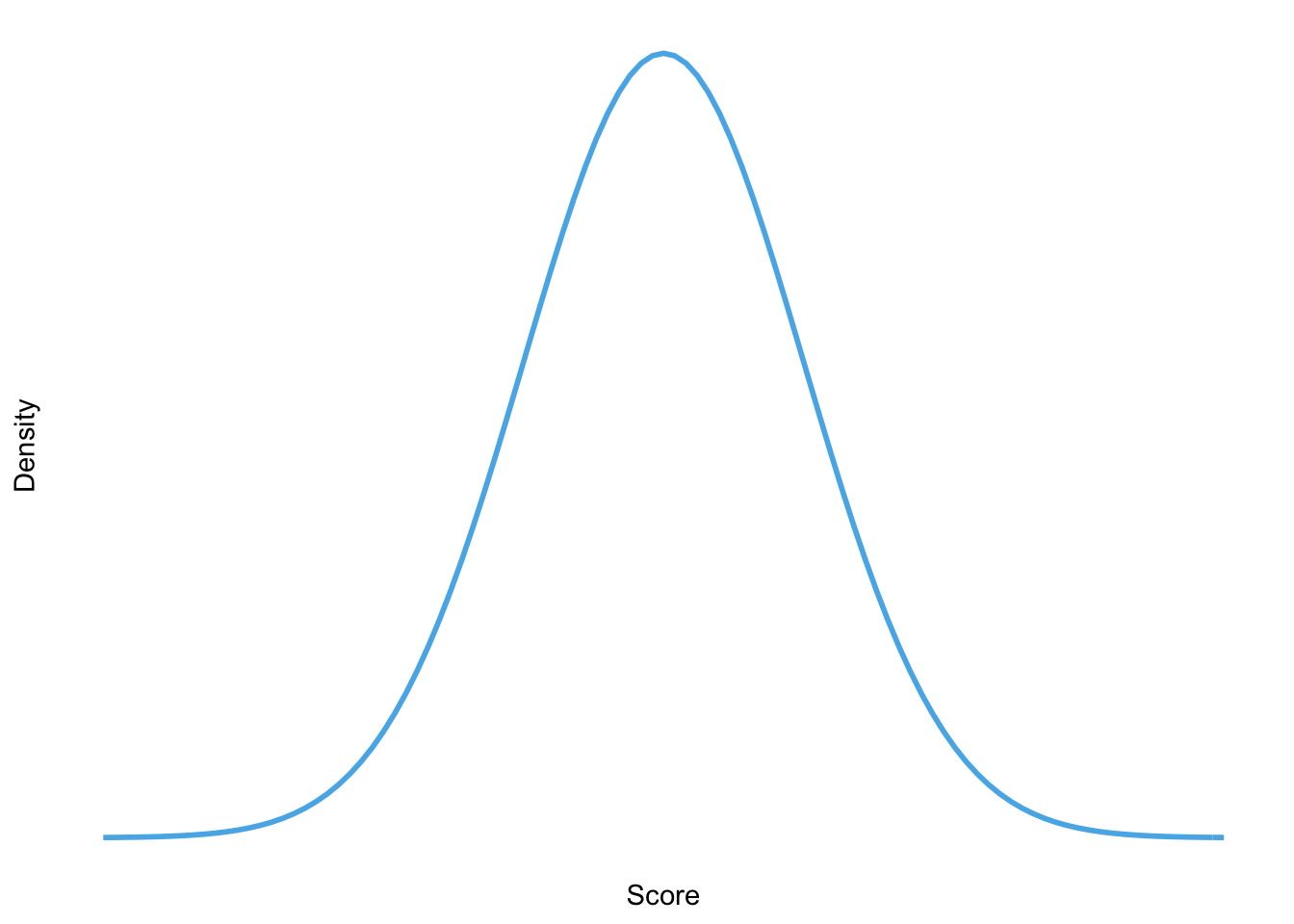
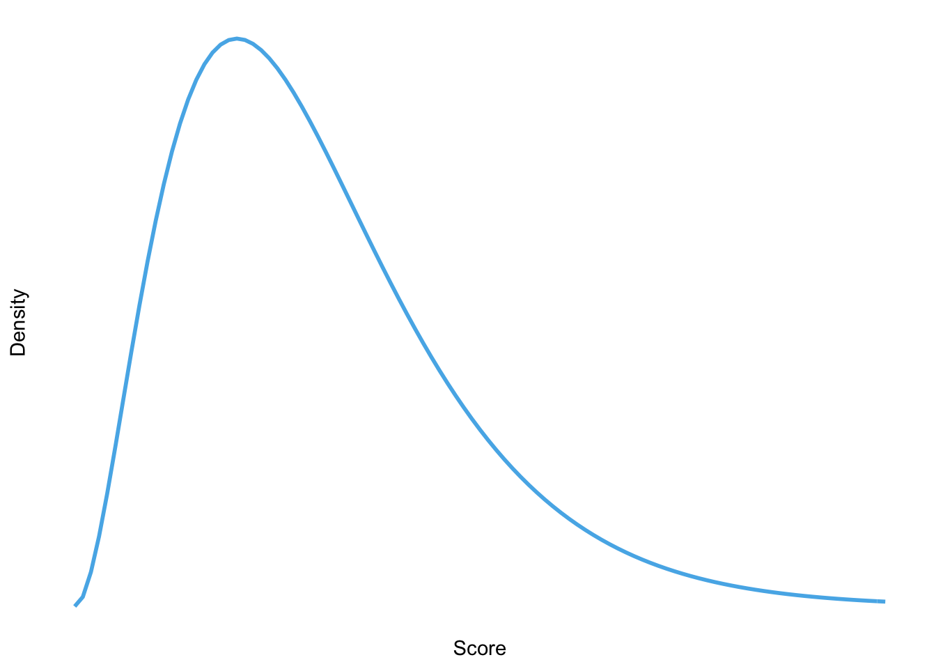
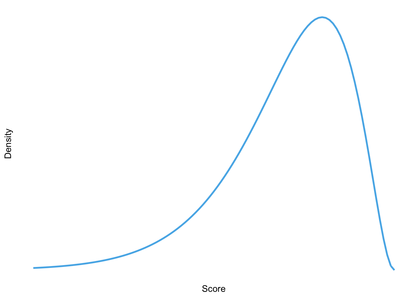
Sketch the shape of a normal distribution, a positively skewed distribution and a negatively skewed distribution.
Normal
Positive skew
Negative skew
Task 2.6
In 2011 I got married and we went to Disney Florida for our honeymoon. We bought some bride and groom Mickey Mouse hats and wore them around the parks. The staff at Disney are really nice and upon seeing our hats would say ‘congratulations’ to us. We counted how many times people said congratulations over 7 days of the honeymoon: 5, 13, 7, 14, 11, 9, 17. Calculate the mean, median, sum of squares, variance and standard deviation of these data.
First compute the mean:
$$ \begin{aligned} \overline{X} &= \frac{\sum_{i=1}^{n} x_i}{n} \\
\ &= \frac{5+13+7+14+11+9+17}{7} \\
\ &= \frac{76}{7} \\
\ &= 10.86 \end{aligned} $$
To calculate the median, first let’s arrange the scores in ascending order: 5, 7, 9, 11, 13, 14, 17. The median will be the (n + 1)/2th score. There are 7 scores, so this will be the 8/2 = 4th. The 4th score in our ordered list is 11.
To calculate the sum of squares, first take the mean from each score, then square this difference, finally, add up these squared values:
| Score | Error (score - mean) | Error squared |
|---|---|---|
| 5 | -5.86 | 34.34 |
| 13 | 2.14 | 4.58 |
| 7 | -3.86 | 14.90 |
| 14 | 3.14 | 9.86 |
| 11 | 0.14 | 0.02 |
| 9 | -1.86 | 3.46 |
| 17 | 6.14 | 37.70 |
So, the sum of squared errors is:
$$ \begin{aligned} \ SS &= 34.34 + 4.58 + 14.90 + 9.86 + 0.02 + 3.46 + 37.70 \\
\ &= 104.86 \end{aligned} $$
The variance is the sum of squared errors divided by the degrees of freedom:
$$ \begin{aligned} \ s^2 &= \frac{SS}{N - 1} \\
\ &= \frac{104.86}{6} \\
\ &= 17.48 \end{aligned} $$
The standard deviation is the square root of the variance:
$$ \begin{aligned} \ s &= \sqrt{s^2} \\
\ &= \sqrt{17.48} \\
\ &= 4.18 \end{aligned} $$
Task 2.7
In this chapter we used an example of the time taken for 21 heavy smokers to fall off a treadmill at the fastest setting (18, 16, 18, 24, 23, 22, 22, 23, 26, 29, 32, 34, 34, 36, 36, 43, 42, 49, 46, 46, 57). Calculate the sums of squares, variance and standard deviation of these data.
To calculate the sum of squares, take the mean from each value, then square this difference. Finally, add up these squared values (the values in the final column). The sum of squared errors is a massive 2685.24.
| Score | Mean | Difference | Difference squared |
|---|---|---|---|
| 18 | 32.19 | -14.19 | 201.36 |
| 16 | 32.19 | -16.19 | 262.12 |
| 18 | 32.19 | -14.19 | 201.36 |
| 24 | 32.19 | -8.19 | 67.08 |
| 23 | 32.19 | -9.19 | 84.46 |
| 22 | 32.19 | -10.19 | 103.84 |
| 22 | 32.19 | -10.19 | 103.84 |
| 23 | 32.19 | -9.19 | 84.46 |
| 26 | 32.19 | -6.19 | 38.32 |
| 29 | 32.19 | -3.19 | 10.18 |
| 32 | 32.19 | -0.19 | 0.04 |
| 34 | 32.19 | 1.81 | 3.28 |
| 34 | 32.19 | 1.81 | 3.28 |
| 36 | 32.19 | 3.81 | 14.52 |
| 36 | 32.19 | 3.81 | 14.52 |
| 43 | 32.19 | 10.81 | 116.86 |
| 42 | 32.19 | 9.81 | 96.24 |
| 49 | 32.19 | 16.81 | 282.58 |
| 46 | 32.19 | 13.81 | 190.72 |
| 46 | 32.19 | 13.81 | 190.72 |
| 57 | 32.19 | 24.81 | 615.54 |
The variance is the sum of squared errors divided by the degrees of freedom ($ N-1 $). There were 21 scores and so the degrees of freedom were 20. The variance is, therefore:
$$ \begin{aligned} \ s^2 &= \frac{SS}{N - 1} \\
\ &= \frac{2685.24}{20} \\
\ &= 134.26 \end{aligned} $$
The standard deviation is the square root of the variance:
$$ \begin{aligned} \ s &= \sqrt{s^2} \\
\ &= \sqrt{134.26} \\
\ &= 11.59 \end{aligned} $$
Task 2.8
Sports scientists sometimes talk of a ‘red zone’, which is a period during which players in a team are more likely to pick up injuries because they are fatigued. When a player hits the red zone it is a good idea to rest them for a game or two. At a prominent London football club that I support, they measured how many consecutive games the 11 first team players could manage before hitting the red zone: 10, 16, 8, 9, 6, 8, 9, 11, 12, 19, 5. Calculate the mean, standard deviation, median, range and interquartile range.
First we need to compute the mean:
$$ \begin{aligned} \overline{X} &= \frac{\sum_{i=1}^{n} x_i}{n} \\
\ &= \frac{10+16+8+9+6+8+9+11+12+19+5}{11} \\
\ &= \frac{113}{11} \\
\ &= 10.27 \end{aligned} $$
Then the standard deviation, which we do as follows:
| Score | Error (score - mean) | Error squared |
|---|---|---|
| 10 | -0.27 | 0.07 |
| 16 | 5.73 | 32.83 |
| 8 | -2.27 | 5.15 |
| 9 | -1.27 | 1.61 |
| 6 | -4.27 | 18.23 |
| 8 | -2.27 | 5.15 |
| 9 | -1.27 | 1.61 |
| 11 | 0.73 | 0.53 |
| 12 | 1.73 | 2.99 |
| 19 | 8.73 | 76.21 |
| 5 | -5.27 | 27.77 |
So, the sum of squared errors is:
$$ \begin{aligned}
\ SS &= 0.07 + 32.80 + 5.17 + 1.62 + 18.26 + 5.17 + 1.62 + 0.53 + 2.98 + 76.17 + 27.80 \\
\ &= 172.18 \\
\end{aligned} $$
The variance is the sum of squared errors divided by the degrees of freedom:
$$ \begin{aligned} \ s^2 &= \frac{SS}{N - 1} \\
\ &= \frac{172.18}{10} \\
\ &= 17.22 \end{aligned} $$
The standard deviation is the square root of the variance:
$$ \begin{aligned} \ s &= \sqrt{s^2} \\
\ &= \sqrt{17.22} \\
\ &= 4.15 \end{aligned} $$
- To calculate the median, range and interquartile range, first let’s arrange the scores in ascending order: 5, 6, 8, 8, 9, 9, 10, 11, 12, 16, 19. The median: The median will be the ($n + 1$)/2th score. There are 11 scores, so this will be the 12/2 = 6th. The 6th score in our ordered list is 9 games. Therefore, the median number of games is 9.
- The lower quartile: This is the median of the lower half of scores. If we split the data at 9 (the 6th score), there are 5 scores below this value. The median of 5 = 6/2 = 3rd score. The 3rd score is 8, the lower quartile is therefore 8 games.
- The upper quartile: This is the median of the upper half of scores. If we split the data at 9 again (not including this score), there are 5 scores above this value. The median of 5 = 6/2 = 3rd score above the median. The 3rd score above the median is 12; the upper quartile is therefore 12 games.
- The range: This is the highest score (19) minus the lowest (5), i.e. 14 games.
- The interquartile range: This is the difference between the upper and lower quartile: $ 12-8 = 4 $ games.
Task 2.9
Celebrities always seem to be getting divorced. The (approximate) length of some celebrity marriages in days are: 240 (J-Lo and Cris Judd), 144 (Charlie Sheen and Donna Peele), 143 (Pamela Anderson and Kid Rock), 72 (Kim Kardashian, if you can call her a celebrity), 30 (Drew Barrymore and Jeremy Thomas), 26 (Axl Rose and Erin Everly), 2 (Britney Spears and Jason Alexander), 150 (Drew Barrymore again, but this time with Tom Green), 14 (Eddie Murphy and Tracy Edmonds), 150 (Renee Zellweger and Kenny Chesney), 1657 (Jennifer Aniston and Brad Pitt). Compute the mean, median, standard deviation, range and interquartile range for these lengths of celebrity marriages.
First we need to compute the mean:
$$ \begin{aligned} \overline{X} &= \frac{\sum_{i=1}^{n} x_i}{n} \\
\ &= \frac{240+144+143+72+30+26+2+150+14+150+1657}{11} \\
\ &= \frac{2628}{11} \\
\ &= 238.91 \end{aligned} $$
Then the standard deviation, which we do as follows:
| Score | Error (score - mean) | Error squared |
|---|---|---|
| 240 | 1.09 | 1.19 |
| 144 | -94.91 | 9007.91 |
| 143 | -95.91 | 9198.73 |
| 72 | -166.91 | 27858.95 |
| 30 | -208.91 | 43643.39 |
| 26 | -212.91 | 45330.67 |
| 2 | -236.91 | 56126.35 |
| 150 | -88.91 | 7904.99 |
| 14 | -224.91 | 50584.51 |
| 150 | -88.91 | 7904.99 |
| 1657 | 1418.09 | 2010979.25 |
So, the sum of squared errors is:
$$ \begin{aligned}
\ SS &= 1.19 + 9007.74 + 9198.55 + 27858.64 + 43643.01 + 45330.28 + 56125.92 + 7904.83 + 50584.10 + 7904.83 + 2010981.83 \\
\ &= 2268540.92 \\ \end{aligned} $$
The variance is the sum of squared errors divided by the degrees of freedom:
$$ \begin{aligned} \ s^2 &= \frac{SS}{N - 1} \\
\ &= \frac{2268540.92}{10} \\
\ &= 226854.09 \end{aligned} $$
The standard deviation is the square root of the variance:
$$ \begin{aligned} \ s &= \sqrt{s^2} \\
\ &= \sqrt{226854.09} \\
\ &= 476.29 \end{aligned} $$
- To calculate the median, range and interquartile range, first let’s arrange the scores in ascending order: 2, 14, 26, 30, 72, 143, 144, 150, 150, 240, 1657. The median: The median will be the (n + 1)/2th score. There are 11 scores, so this will be the 12/2 = 6th. The 6th score in our ordered list is 143. The median length of these celebrity marriages is therefore 143 days.
- The lower quartile: This is the median of the lower half of scores. If we split the data at 143 (the 6th score), there are 5 scores below this value. The median of 5 = 6/2 = 3rd score. The 3rd score is 26, the lower quartile is therefore 26 days.
- The upper quartile: This is the median of the upper half of scores. If we split the data at 143 again (not including this score), there are 5 scores above this value. The median of 5 = 6/2 = 3rd score above the median. The 3rd score above the median is 150; the upper quartile is therefore 150 days.
- The range: This is the highest score (1657) minus the lowest (2), i.e. 1655 days.
- The interquartile range: This is the difference between the upper and lower quartile: $ 150 - 26 = 124$ days.
Task 2.10
Repeat Task 9 but excluding Jennifer Anniston and Brad Pitt’s marriage. How does this affect the mean, median, range, interquartile range, and standard deviation? What do the differences in values between Tasks 9 and 10 tell us about the influence of unusual scores on these measures?
First let’s compute the new mean:
$$ \begin{aligned} \overline{X} &= \frac{\sum_{i=1}^{n} x_i}{n} \\
\ &= \frac{240+144+143+72+30+26+2+150+14+150}{11} \\
\ &= \frac{971}{11} \\
\ &= 97.1 \end{aligned} $$
The mean length of celebrity marriages is now 97.1 days compared to 238.91 days when Jennifer Aniston and Brad Pitt’s marriage was included. This demonstrates that the mean is greatly influenced by extreme scores.
Let’s now calculate the standard deviation excluding Jennifer Aniston and Brad Pitt’s marriage:
| Score | Error (score - mean) | Error squared |
|---|---|---|
| 240 | 142.9 | 20420.41 |
| 144 | 46.9 | 2199.61 |
| 143 | 45.9 | 2106.81 |
| 72 | -25.1 | 630.01 |
| 30 | -67.1 | 4502.41 |
| 26 | -71.1 | 5055.21 |
| 2 | -95.1 | 9044.01 |
| 150 | 52.9 | 2798.41 |
| 14 | -83.1 | 6905.61 |
| 150 | 52.9 | 2798.41 |
So, the sum of squared errors is:
$$ \begin{aligned} \ SS &= 20420.41 + 2199.61 + 2106.81 + 630.01 + 4502.41 + 5055.21 + 9044.01 + 2798.41 + 6905.61 + 2798.41 \\
\ &= 56460.90 \end{aligned} $$
The variance is the sum of squared errors divided by the degrees of freedom:
$$ \begin{aligned} s^2 &= \frac{SS}{N - 1} \\
&= \frac{56460.90}{9} \\
&= 6273.43 \end{aligned} $$
The standard deviation is the square root of the variance:
$$ \begin{aligned} s &= \sqrt{s^2} \\
&= \sqrt{6273.43} \\
&= 79.21 \end{aligned} $$
From these calculations we can see that the variance and standard deviation, like the mean, are both greatly influenced by extreme scores. When Jennifer Aniston and Brad Pitt’s marriage was included in the calculations (see Smart Alex Task 9), the variance and standard deviation were much larger, i.e. 226854.09 and 476.29 respectively.
- To calculate the median, range and interquartile range, first, let’s again arrange the scores in ascending order but this time excluding Jennifer Aniston and Brad Pitt’s marriage: 2, 14, 26, 30, 72, 143, 144, 150, 150, 240.
- The median: The median will be the (n + 1)/2 score. There are now 10 scores, so this will be the 11/2 = 5.5th. Therefore, we take the average of the 5th score and the 6th score. The 5th score is 72, and the 6th is 143; the median is therefore 107.5 days.
- The lower quartile: This is the median of the lower half of scores. If we split the data at 107.5 (this score is not in the data set), there are 5 scores below this value. The median of 5 = 6/2 = 3rd score. The 3rd score is 26; the lower quartile is therefore 26 days.
- The upper quartile: This is the median of the upper half of scores. If we split the data at 107.5 (this score is not actually present in the data set), there are 5 scores above this value. The median of 5 = 6/2 = 3rd score above the median. The 3rd score above the median is 150; the upper quartile is therefore 150 days.
- The range: This is the highest score (240) minus the lowest (2), i.e. 238 days. You’ll notice that without the extreme score the range drops dramatically from 1655 to 238 – less than half the size.
- The interquartile range: This is the difference between the upper and lower quartile: $ 150−26 = 124 $ days of marriage. This is the same as the value we got when Jennifer Aniston and Brad Pitt’s marriage was included. This demonstrates the advantage of the interquartile range over the range, i.e. it isn’t affected by extreme scores at either end of the distribution